Maps for Milvus milvus

Alexander Dunkel, Leibniz Institute of Ecological Urban and Regional Development, Transformative Capacities & Research Data Centre (IÖR-FDZ)

Publication:
Dunkel, A., Burghardt, D. (2024). Assessing perceived landscape change from opportunistic spatio-temporal occurrence data. Land 2024

Summary

In this section we intend to share additional notebooks on various topics in spatial visualisation, prepared by colleagues for specific projects or publications.

This sample notebook on exploration of “Milvus milvus” observations (Red Kite) on iNaturalist has been prepared and shared in a data repository specifically for replicating figures in a publication (Dunkel & Burghardt 2024(Dunkel and Burghardt 2024)). It is shared as is, as an example to document a real publication workflow. We do not provide any dependency setup. This notebook was last updated on Aug-19-2023, Carto-Lab Docker, version 0.14.0. If you want to replicate this notebook, either install the dependencies manually or use the appropriate Carto-Lab Docker container archive version which includes all dependencies.

Last updated: Aug-19-2023, Carto-Lab Docker Version 0.14.0

Visualization of spatial patterns for Milvus milvus observations (Flickr, iNaturalist).

Preparations

import os, sys
from pathlib import Path
import psycopg2
import geopandas as gp
import pandas as pd
import seaborn as sns
import numpy as np
import hdbscan
import calendar
import matplotlib
import matplotlib.pyplot as plt
import matplotlib.dates as mdates
import matplotlib.ticker as mticker
import matplotlib.patheffects as pe
import matplotlib.patches as mpatches
from typing import List, Tuple, Dict, Optional, Any
from IPython.display import clear_output, display, HTML
from datetime import datetime
from pyproj import Transformer
from shapely.geometry import box

module_path = str(Path.cwd().parents[0] / "py")
if module_path not in sys.path:
    sys.path.append(module_path)
from modules.base import tools, hll
from modules.base.hll import union_hll, cardinality_hll

%load_ext autoreload
%autoreload 2

The autoreload extension is already loaded. To reload it, use:
  %reload_ext autoreload

OUTPUT = Path.cwd().parents[0] / "out"       # output directory for figures (etc.)
WORK_DIR = Path.cwd().parents[0] / "tmp"     # Working directory

(OUTPUT / "figures").mkdir(exist_ok=True)
(OUTPUT / "svg").mkdir(exist_ok=True)
WORK_DIR.mkdir(exist_ok=True)

Plot styling

plt.style.use('default')

CRS_WGS = "epsg:4326" # WGS1984
CRS_PROJ = "esri:54009" # Mollweide
# CRS_PROJ = "esri:102014" # Lambert Conformal Conic

Define Transformer ahead of time with xy-order of coordinates

PROJ_TRANSFORMER = Transformer.from_crs(
    CRS_WGS, CRS_PROJ, always_xy=True)

Set global font

plt.rcParams['font.family'] = 'serif'
plt.rcParams['font.serif'] = ['Times New Roman'] + plt.rcParams['font.serif']

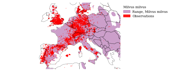
Load Milvus range

This is the habitat range calculated by iNaturalist observations. The area is currently very broad and includes many locations, where Milvus milvus will be only very seldom observable.

DATA_FOLDER = Path.cwd().parents[0] / "00_data" / "milvus"
range_kml = DATA_FOLDER / "range.kml"

from fiona.drvsupport import supported_drivers
supported_drivers['KML'] = 'rw'

df = gp.read_file(range_kml, driver='KML', ignore_geometry=False)
print(df.crs)

epsg:4326

save to Geopackage, for archive purposes

df.to_file(
    OUTPUT/ 'Milvusmilvus_range.gpkg', driver='GPKG', layer='Milvus milvus')  

project to Mollweide

gdf_range = df.to_crs(CRS_PROJ)

ax = gdf_range.plot()
ax.set_axis_off()

Load Milvus milvus observations

Load observation data. This data was requested with the iNaturalist Export tool, based on a species search for Milvus. Milvus includes 2 species.

df = pd.read_csv(DATA_FOLDER / "observations-350501.csv")

df.head()

	id	observed_on_string	observed_on	time_observed_at	time_zone	user_id	user_login	user_name	created_at	updated_at	...	geoprivacy	taxon_geoprivacy	coordinates_obscured	positioning_method	positioning_device	species_guess	scientific_name	common_name	iconic_taxon_name	taxon_id
0	7793	May 22, 2010 13:59	2010-05-22	2010-05-22 12:59:00 UTC	London	446	kevinandseri	NaN	2010-07-10 09:15:17 UTC	2016-06-22 18:30:14 UTC	...	NaN	open	False	NaN	NaN	Red Kite	Milvus milvus	Rotmilan	Aves	5267
1	9495	2011-01-01 11:29	2011-01-01	2011-01-01 11:29:00 UTC	London	351	zabdiel	John Proctor	2011-01-01 11:31:50 UTC	2016-06-22 18:32:46 UTC	...	NaN	open	False	NaN	NaN	Red Kite	Milvus milvus	Rotmilan	Aves	5267
2	9496	2011-01-01 11:42	2011-01-01	2011-01-01 11:42:00 UTC	London	351	zabdiel	John Proctor	2011-01-01 11:43:09 UTC	2016-06-22 18:32:46 UTC	...	NaN	open	False	NaN	NaN	red kite	Milvus milvus	Rotmilan	Aves	5267
3	14694	2011-04-17	2011-04-17	NaN	London	654	spookypeanut	NaN	2011-04-17 18:18:12 UTC	2016-06-22 18:44:11 UTC	...	NaN	open	False	NaN	NaN	Red Kite	Milvus milvus	Rotmilan	Aves	5267
4	50134	2011-10-05	2011-10-05	NaN	Berlin	4130	michael	Michael	2012-02-01 19:59:12 UTC	2016-06-22 19:39:03 UTC	...	NaN	open	False	NaN	NaN	Milvus milvus	Milvus milvus	Rotmilan	Aves	5267

5 rows × 39 columns

df.columns

Index(['id', 'observed_on_string', 'observed_on', 'time_observed_at',
       'time_zone', 'user_id', 'user_login', 'user_name', 'created_at',
       'updated_at', 'quality_grade', 'license', 'url', 'image_url',
       'sound_url', 'tag_list', 'description', 'num_identification_agreements',
       'num_identification_disagreements', 'captive_cultivated',
       'oauth_application_id', 'place_guess', 'latitude', 'longitude',
       'positional_accuracy', 'private_place_guess', 'private_latitude',
       'private_longitude', 'public_positional_accuracy', 'geoprivacy',
       'taxon_geoprivacy', 'coordinates_obscured', 'positioning_method',
       'positioning_device', 'species_guess', 'scientific_name', 'common_name',
       'iconic_taxon_name', 'taxon_id'],
      dtype='object')

milvus_inat = gp.GeoDataFrame(
    df, geometry=gp.points_from_xy(df.longitude, df.latitude), crs=CRS_WGS)
milvus_inat.to_crs(CRS_PROJ, inplace=True)

Load world countries geometry

world = tools.get_shapes("world", shape_dir=OUTPUT / "shapes")

Already exists

world.to_crs(CRS_PROJ, inplace=True)

bbox_europe = -25, 35, 35, 59
# convert to Mollweide
minx, miny = PROJ_TRANSFORMER.transform(
    bbox_europe[0], bbox_europe[1])
maxx, maxy = PROJ_TRANSFORMER.transform(
    bbox_europe[2], bbox_europe[3])

RANGE_COLOR = "#810f7c"
OBSERVATION_COLOR = "red"

Create legend manually

range_patch = mpatches.Patch(
    color=RANGE_COLOR,
    label='Range, Milvus milvus', alpha=0.4)
obs_patch = mpatches.Patch(
    color=OBSERVATION_COLOR,
    label='Observations', alpha=0.9)
legend_entries = [range_patch, obs_patch]
legend_kwds = {
    "bbox_to_anchor": (1.0, 1),
    "loc":'upper left',
    "fontsize":8, "frameon":False,
    "title":"Milvus milvus", "title_fontsize":8,
    "alignment":"left"}

def plot_map(
    gdf: gp.GeoDataFrame, x_lim: [Tuple[float, float]] = None, y_lim: [Tuple[float, float]] = None,
    gdf_range: gp.GeoDataFrame = None, world: gp.GeoDataFrame = None,
    legend_entries: List[mpatches.Patch] = None, legend_kwds: Dict[str, Any]  = None, 
    range_color: str = RANGE_COLOR, observation_color: str = OBSERVATION_COLOR, fig_size: Tuple[int, int] = None,
    return_ax: bool = None):
    """Plot a point map with legend and optional range-shape"""
    if fig_size is None:
        fig_size = (6, 9)
    fig, ax = plt.subplots(1, 1, figsize=fig_size)
    if gdf_range is not None:
        gdf_range.plot(
            ax=ax,
            facecolor=range_color,
            edgecolor=None,
            alpha=0.4)
    gdf.plot(
        ax=ax,
        markersize=.1,
        facecolor=observation_color,
        edgecolor=None,
        alpha=0.9)
    if world is not None:
        world.plot(
            ax=ax, color='none', edgecolor='black', linewidth=0.3)
    if not None in [x_lim, y_lim]:
        ax.set_xlim(*x_lim)
        ax.set_ylim(*y_lim)
    ax.axis('off')
    if not None in [legend_entries, legend_kwds]:
        ax.legend(
            handles=legend_entries, **legend_kwds)
    fig.tight_layout()
    if return_ax:
        return fig, ax
    fig.show()

fig, ax = plot_map(
    milvus_inat, x_lim=(minx, maxx), y_lim=(miny, maxy), 
    gdf_range=gdf_range, world=world, legend_entries=legend_entries, 
    legend_kwds=legend_kwds, return_ax=True)
fig.show()
tools.save_fig(fig, output=OUTPUT, name="milvus_inat_europe")

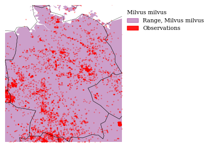
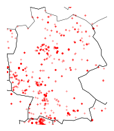
Zoom in

bbox_germany = world[world.index == "Germany"].bounds.values.squeeze()
minx, miny = bbox_germany[0], bbox_germany[1]
maxx, maxy = bbox_germany[2], bbox_germany[3]

plot_map(
    milvus_inat, x_lim=(minx, maxx), y_lim=(miny, maxy), 
    gdf_range=gdf_range, world=world, 
    legend_entries=legend_entries, legend_kwds=legend_kwds, fig_size=(6,3))

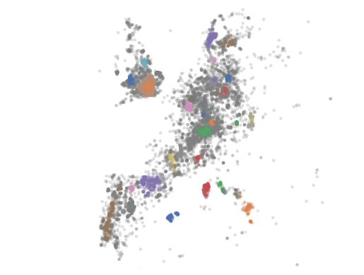
Find clusters (HDBSCAN)

We just want to see distribution and major clusters. A more interactive approach is shown by João Paulo Figueira’s Geographic Clustering with HDBSCAN

data = np.array(list(zip(df.longitude, df.latitude)))

X = np.radians(data) # convert the list of lat/lon coordinates to radians
earth_radius_km = 6371
epsilon = 0.005 / earth_radius_km # calculate 5 meter epsilon threshold

clusterer = hdbscan.HDBSCAN(min_cluster_size=100, metric='haversine').fit(X)

color_palette = sns.color_palette('deep', len(clusterer.labels_))
cluster_colors = [color_palette[x] if x >= 0
                  else (0.5, 0.5, 0.5)
                  for x in clusterer.labels_]
cluster_member_colors = [sns.desaturate(x, p) for x, p in
                         zip(cluster_colors, clusterer.probabilities_)]
fig, ax = plt.subplots()
ax.scatter(*data.T, s=10, linewidth=0, c=cluster_member_colors, alpha=0.25)
ax.set_xlim(bbox_europe[0], bbox_europe[1])
ax.set_ylim(bbox_europe[2], bbox_europe[3])
ax.axis('off')
fig.show()

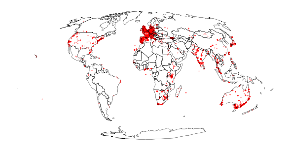
Load Milvus milvus Flickr observations (worldwide)

flickr_observations = DATA_FOLDER / "2022-02-17_milvusmilvus.csv"

df = pd.read_csv(flickr_observations)

Time format: see Python strftime cheatsheet

load_kwargs = {
    "index_col":'datetime', 
    "parse_dates":{'datetime':["post_create_date"]},
    "date_format":'%Y-%m-%d %H:%M:%S',
    "keep_date_col":'False',
    "usecols":["post_guid", "post_create_date", "latitude", "longitude"]
}

df = pd.read_csv(flickr_observations, **load_kwargs)

df.head(1)

	post_guid	latitude	longitude	post_create_date
datetime
2012-10-01	XSQGXtc9wWIHX6XiEtdaOqgKPURZ7tZtIRere0IA7wQ	52.246984	-3.628835	2012-10-01

milvus_flickr = gp.GeoDataFrame(
    df, geometry=gp.points_from_xy(df.longitude, df.latitude), crs=CRS_WGS)
milvus_flickr.to_crs(CRS_PROJ, inplace=True)

plot

plot_map(
    milvus_flickr, world=world)

plot_map(
    milvus_flickr, world=world, x_lim=(minx, maxx), y_lim=(miny, maxy), fig_size=(4,2))

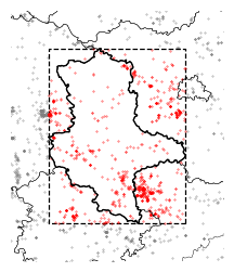
Saxony-Anhalt

According to Nicolai, Mammen & Kolbe (2017), the highest population of the Red Kite is found in Saxony-Anhalt.

Nicolai, B., Mammen, U., & Kolbe, M. (2017). Long-term changes in population and habitat selection of Red Kite Milvus milvus in the region with the highest population density. VOGELWELT 137: 194–197 (2017)

Below, we visualize this area, merging Flickr and iNaturalist observations.

shapes = tools.get_shapes("de", shape_dir=OUTPUT / "shapes", project_wgs84=False)

Loaded 5.10 MB of 5.11 (100%)..
Extracting zip..
Retrieved vg2500_12-31.utm32s.shape.zip, extracted size: 0.73 MB

We want to filter by Saxony-Anhalt with a buffer of 100 km

geom_saxonya = shapes[shapes.index == "Sachsen-Anhalt"]

Get bounds of Saxony-Anhalt

geom_saxonya_bbox = box(*geom_saxonya.total_bounds)

Project and concat Flickr and iNaturalist observations

milvus_gdf = pd.concat(
    [milvus_flickr.to_crs(shapes.crs), milvus_inat.to_crs(shapes.crs)])

Clip observations to bounds of Saxony-Anhalt (only iNat, as there are only 4 Flickr obervations of Milvus in the focus region)

Note: We could also use gp.overlay() here, e.g.:

gdf_select = gp.overlay(
    milvus_gdf, geom_saxonya_bbox,
    how='intersection')

gdf_select = gp.clip(milvus_inat.to_crs(shapes.crs), mask=geom_saxonya_bbox)

len(gdf_select)

856

Set bounds of Saxony-Anhalt as plotting limits

bbox_saxonya = geom_saxonya.bounds.values.squeeze()

bbox_saxonya

array([ 607181.85913772, 5647848.4600198 ,  789161.6620191 ,
       5880180.07203066])

minx, miny = bbox_saxonya[0], bbox_saxonya[1]
maxx, maxy = bbox_saxonya[2], bbox_saxonya[3]

bbox_layer = gp.GeoDataFrame(index=[0], crs=shapes.crs.to_epsg(), geometry=[geom_saxonya_bbox])

fig, ax = plt.subplots(1, 1, figsize=(5, 3))
ax = milvus_gdf.plot(
    ax=ax,
    markersize=.1,
    facecolor="grey",
    edgecolor=None,
    alpha=0.9)
ax = bbox_layer.plot(
    ax=ax, color='white', edgecolor='black', 
    linewidth=0.9, linestyle='dashed')
ax = gdf_select.plot(
    ax=ax,
    markersize=.1,
    facecolor=OBSERVATION_COLOR,
    edgecolor=None,
    alpha=0.9)
ax = shapes.plot(
    ax=ax, color='none', edgecolor='black', linewidth=0.3)
ax = shapes[shapes.index == "Sachsen-Anhalt"].plot(
    ax=ax, color='none', edgecolor='black', linewidth=1)
buf = 50000 # 50km
ax.axis('off')
ax.set_xlim((minx-buf, maxx+buf))
ax.set_ylim((miny-buf, maxy+buf))
fig.show()

tools.save_fig(fig, output=OUTPUT, name="focus_region")

WGS bounds:

bbox_layer.to_crs(CRS_WGS).bounds.values.squeeze()

array([10.52659544, 50.90971941, 13.30916778, 53.0603523 ])

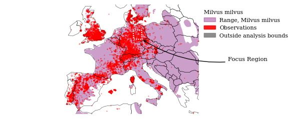
Update our Europe plot with the bounds of the close-up region.

bbox_europe = -25, 35, 35, 59
# convert to Mollweide
minx, miny = PROJ_TRANSFORMER.transform(
    bbox_europe[0], bbox_europe[1])
maxx, maxy = PROJ_TRANSFORMER.transform(
    bbox_europe[2], bbox_europe[3])

Update legend

outside_patch = mpatches.Patch(
    # color="tab:blue", # default matplotlib blue
    color="grey",
    label='Outside analysis bounds', alpha=0.9)
if len(legend_entries) > 2:
    legend_entries.pop()
legend_entries.append(outside_patch)

bbox_layer.loc[0, "name"] = "Focus Region"

label_off = {
    "Focus Region":(-2000000, 500000),
}
label_rad = {
    "Focus Region":-0.2,
}

Annotatipn arrow ending at lower-right corner

lower_right = (
    bbox_layer.to_crs(CRS_PROJ).bounds.values.squeeze()[2],
    bbox_layer.to_crs(CRS_PROJ).bounds.values.squeeze()[1])

fig, ax = plot_map(
    milvus_inat, x_lim=(minx, maxx), y_lim=(miny, maxy), 
    gdf_range=gdf_range, world=world, 
    legend_entries=legend_entries, legend_kwds=legend_kwds, return_ax=True)
ax = bbox_layer.to_crs(CRS_PROJ).plot(
    ax=ax, color='none', edgecolor='white', 
    linewidth=1.5, linestyle=(0, (1,1)))
tools.annotate_locations(
    gdf=bbox_layer, ax=ax, label_off=label_off, label_rad=label_rad, 
    text_col="name", arrowstyle='->', arrow_col='black', fontsize="small",
    coords=lower_right)
fig.show()

tools.save_fig(fig, output=OUTPUT, name="milvus_inat_europe_annotated")

Create notebook HTML

References

[1]

Alexander Dunkel and Dirk Burghardt. Assessing Perceived Landscape Change from Opportunistic Spatiotemporal Occurrence Data. Land, 13(7):1091, July 2024. URL: https://www.mdpi.com/2073-445X/13/7/1091 (visited on 2024-07-22), doi:10.3390/land13071091.