Descriptive Statistics

Descriptive Statistics#

To get an overview of the data, descriptive statistics are used. These include values such as the range, median, and mean. They will help to observe the central tendency, identify outliers, and understand the overall behavior of the data.

For this reason, the `Pandas’ library added.

from pathlib import Path
import pandas as pd
import geopandas as gp

INPUT = Path.cwd().parents[0] / "00_data"
gdb_path = INPUT / "Biotopwerte_Dresden_2018.gdb"

Statistical Summary#

The data of interest is loaded into the environment.

data = gp.read_file(gdb_path, layer="Biotopwerte_Dresden_2018")

/opt/conda/envs/worker_env/lib/python3.13/site-packages/pyogrio/raw.py:198: RuntimeWarning: organizePolygons() received a polygon with more than 100 parts. The processing may be really slow.  You can skip the processing by setting METHOD=SKIP, or only make it analyze counter-clock wise parts by setting METHOD=ONLY_CCW if you can assume that the outline of holes is counter-clock wise defined
  return ogr_read(

Then the describe function of Pandas is used to create a summary.

The describe function

By default, the describe function creates a summary for the columns with numerical format.

The statistical summary generated by describe function for each Numerical column:

Count: Number of values
Mean: Average of the values
Std : spread of the data (Standard deviation)
Min: The minimum value
25%: lower quartile
50%: median
75%: upper quartile
Max: The Maximum value

num_statistics = data.describe()
print(num_statistics)

        Biotpkt2018   Shape_Length    Shape_Area
count  33923.000000   33923.000000  3.392300e+04
mean       8.804984     590.458984  9.662175e+03
std        4.784322    6169.780269  4.671589e+04
min        0.000000       0.011841  5.620002e-06
25%        5.271487     136.936684  2.437363e+02
50%        7.000000     306.549587  2.016611e+03
75%       12.594189     564.009207  8.515168e+03
max       20.164493  612646.861125  3.249895e+06

describe(include=’all’)

To obtain the summary statistics for all columns, including both numerical and string formats, the describe function should be called with the include='all' parameter.

The additional statistical summary generated by describe(include='all') for string Columns:

unique: number of distinct values
top: most frequent value (mode)
Freq: frequency of the top value

statistics = data.describe(include='all')
print(statistics)

NaN values description!

In some cases, there are NaN values in the columns. These could indicate missing values or situations where a statistical calculation is not possible for certain columns, especially for text-based data.

ex: metrics such as mean, min, and max do not apply to string columns!

Statistical Analysis#

Based on the attributes in the dataset which mentioned in Selecting and Filtering Data Chapter, the CLC_st1 includes the landcover classifications.

To find the area allocated to each group of landcovers, the dataset should be groped by the unique landcovers and calculate the sum of the areas.

reset_index!

In case the output is going to be used as a DataFrame for further analysis, using reset_index to create a new index for calculated features is recommended.

The output shows the area allocated to each landcover with specific indexes.

Based on the output for example 2.637234e+05 equal to 263723.4 square meters allocated to the landcover class of 221, which is the Vineyard class.

clc_areas = data.groupby("CLC_st1")["Shape_Area"]\
                .sum()\
                .reset_index()
print (clc_areas)

Also to see the minimum, maximum and mean value of the covered areas by each landcover class:

areas_range = data.groupby('CLC_st1')['Shape_Area']\
                  .agg(['min', 'max', 'mean'])\
                  .reset_index()
print(areas_range)

It is also possible to convert the area column from square meters to hectares. In the output, it shows that more than 26 hectares belong to the code 221, Vineyards.

clc_areas["Shape_Area"] = clc_areas["Shape_Area"] / 10000  
print(clc_areas)

To find the percentage that belongs to each class:

First, the total area of the landcovers calculated, and then the percentage is calculated, and stored in a column called share in the same dataset.

The following output shows that for example, 0.08% of the area covered by this dataset belongs to the code 221, Vineyards.

total_area = clc_areas["Shape_Area"].sum()
clc_areas["share"] = (clc_areas["Shape_Area"] / total_area) * 100

print(total_area)
print(clc_areas)

To find the summary of the forest areas, the area covered by these landcovers is calculated which includes the classification codes of 311,312 and 313.

The landcover codes are selected using the isin method.

total_forest = data[data['CLC_st1']\
                    .isin(['311', '312', '313'])]['Shape_Area']\
                    .sum()
print (total_forest)

75237414.90073195

To compute the average biodiversity value across all forest areas:

mean_biodiversity = data[data['CLC_st1']\
                        .isin(['311', '312', '313'])]['Biotpkt2018']\
                        .mean()
print(mean_biodiversity)

16.5030688377192

Data Visualization#

To better understand the data, using a plot can offer a clearer visual summary of the data in each column.

Using matplotlib library with various packages allows for the creation of helpful visualizations.

import matplotlib.pyplot as plt

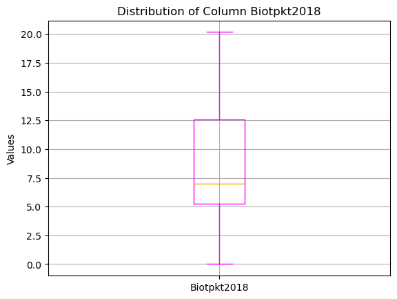
ex: box plot is a great way to quickly review the max, min, median, and quartiles of a dataset.

It is just needed to call the kind of the plot which is needed, for the required column of the dataset.

data['Biotpkt2018'].plot(kind='box',
                        color= 'magenta', 
                        medianprops=dict(color='orange'))

plt.title('Distribution of Column Biotpkt2018')
plt.ylabel('Values') 

plt.grid(True)
plt.show()

../_images/feb276dfa6836a912b43ed98676697eeac3a26d05489b103825ac25b9e4d0f2a.png

More Plots?

To find the most suitable plot based on the needs of the project, matplotlib website offers a wide range of plot types with different customization options.

For effectively visualizing the distribution of continuous data and frequency of data across consecutive intervals also the histograms can be used.

HISTOGRAM

Histograms are just able to represent the frequency of numeric values.

In case the type of the attribute is string like here for landcover classes, for showing frequency there are 2 methods:

Data should be converted to numeric values.
Calculate the frequency of the data as it explained in the Selecting and Filtering chapter, and then use bar chart for plot.

Converting string values to numeric values can be done using the astype method.

numeric_column= data['CLC_st1'].astype(float)

Or using the to_numeric method from Pandas package.

numeric_column= pd.to_numeric(data['CLC_st1'])

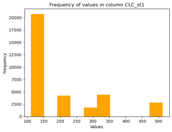
ex: The output shows that in the column CLC_st1 of the dataset, more than 20000 records belong to the landcover codes between 100 and 150.

This range includes the codes 111, 112, 121, 122, 123, 124, 131, 132, 133, 141, and 142 that based on the code interpretation belong to the Artificial Surfaces like Urban fabrics, Industrial, commercial, transport units, mine, dump, construction sites and non-agricultural vegetated areas.

numeric_column.plot(kind='hist', color= 'orange')
plt.title('Frequency of values in column CLC_st1')
plt.xlabel('Values') 
plt.show()

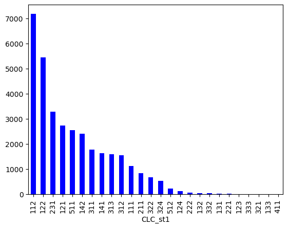
../_images/7f227a179bff1f8c84092d43efb99a3854055bb9134e626605f3a2a396a3d632.png

Or the output using the bar charts with string data and calculating the frequency of the data shows the frequency for each single landcover code.

ex: more than 7000 records in the dataset are related to the code 112 which represents the Discontinuous urban fabric.

a = data['CLC_st1'].value_counts()
a.plot(kind='bar', color='blue')  

<Axes: xlabel='CLC_st1'>

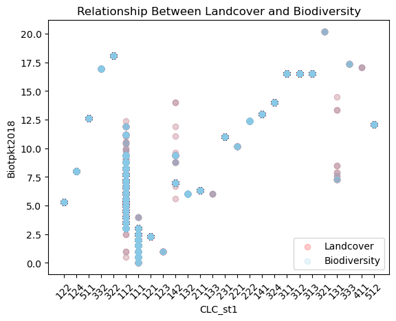
../_images/7d469db5708cc8365c9d49e610df77bc7f871d0c90074e27a3c433637601e101.png

Also if the relationship between two variables in a dataset is important, plots such as scatter plot can be helpful for visualizing and understanding the relation.

ex: in the following output, all the records for the landcover class with code 122, have the same biodiversity value of around 5 but for code 111, different biodiversity values are recorded.

plt.scatter(data['CLC_st1'],
            data['Biotpkt2018'], 
            alpha=0.2, 
            color='red', 
            label='Landcover')

plt.scatter(data['CLC_st1'], 
            data['Biotpkt2018'], 
            alpha=0.2, 
            color='skyblue', 
            label='Biodiversity')


plt.title("Relationship Between Landcover and Biodiversity")
plt.xlabel('CLC_st1')
plt.ylabel('Biotpkt2018')
plt.legend()
plt.xticks(rotation=45)
plt.show()

../_images/0960f8c1daa3cb8b9307a2fd366c11d4cbe4c7918ef0bd8878d07d1fe27c9994.png