Data Retrieval: GBIF & LAND#
Summary
In this section, we will retrieve biodiversity data from GBIF/LAND.
This section covers:
Understanding the GBIF API, including the GBIF Species API and the GBIF Occurrence API
Mapping species data
Write advanced API queries
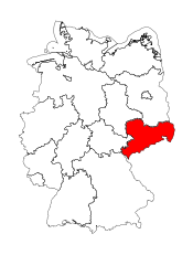
Restrict queries to specific geographic areas (e.g., Saxony).
Handle API limitations and optimize large data retrieval.
Format spatial queries using bounding boxes and WKT polygons.
GBIF API Reference#

Fig. 5 GBIF API Reference (https://techdocs.gbif.org/en/openapi/).#
LAND uses the GBIF Application Programming Interface (API) to provide standardized ways to access biodiversity data.
Retrieving data from APIs requires a specific syntax, which varies for each service. Here are two key concepts:
Endpoint: APIs commonly provide URLs (endpoints) that return structured data (e.g., in JSON format). The base URL for the GBIF API is https://api.gbif.org/.
Authentication: Some APIs require authentication (such as API keys or OAuth tokens), while others - like GBIF- allow limited access without authentication.
How do I know how to work with GBIF API?
Good APIs have a documentation that explains how to use the specific API. It provides details on available endpoints, request methods (e.g., GET, POST), required parameters, and response formats (e.g., JSON, XML), often including code examples and testing tools. Good documentation helps developers to interact with the API efficiently.
The GBIF API Reference documentation is well-structured and divided into several sections. GGBIF uses a RESTful API, which can be accessed through structured URLs. A great feature of this documentation is that it’s built using Swagger, an interactive API framework. Swagger-based API pages allow users to test API queries directly in the browser, making it easier to understand how they work.
Using the GBIF Species API#
Finding a species’ scientific name#
Let’s say we only have a species’ common name — such as English Sparrow, which is also known as House Sparrow - and want to find its scientific name. The scientific name is essential for accurate data retrieval, as common names vary across languages and regions.
We can search for the scientific name manually on Google or the GBIF species search, but a more efficient approach is to use the GBIF Species API.
Using the GBIF Species API in the browser
The GBIF Species API section allows to try the API directly in a web browser.
Go to https://techdocs.gbif.org/en/openapi/v1/species#/Searching%20names/searchNames and use the general species search for “English Sparrow”.
Enter
English Sparrowin the parameter field labeledq, which has the explaination: “The value for this parameter can be a simple word or a phrase. Wildcards are not supported” (Hint: The parameter field is located in the middle of the webpage).
We also specify a dataset to check this taxon. In this case, we use the base GBIF Backbone Taxonomy.
Important caveat: The ambiguity of common names in taxonomic mapping
The next step, where we map the common name “English sparrow” to the scientific name Passer domesticus using the GBIF API, is a simplified example for illustrative purposes in this workshop.
In real-world explorative analytics, this mapping requires careful scrutiny. Common names can be highly ambiguous and may refer to different species depending on region, language, or local usage.
For instance, the German word “Sperlinge” (sparrows) can encompass multiple species, notably the House Sparrow (Passer domesticus) and the Eurasian Tree Sparrow (Passer montanus). These two species have distinct habitat preferences, population trends, and ecological roles. A naive mapping without awareness of this distinction could lead to flawed analyses and conclusions.
For a practical example of how to approach taxonomic reconciliation with more rigor, including techniques for fuzzy matching and merging data from sources like iNaturalist, please refer to this excellent resource: Link iNaturalist observations to TRY by Wolf et al. (2022).
Retrieving GBIF Species API in Python#
We can also query the API directly using Python:
import requests

# Define search parameters
SPECIES_COMMON_NAME = "English Sparrow"
GBIF_DATASET_KEY = "d7dddbf4-2cf0-4f39-9b2a-bb099caae36c"

# Construct API URL
query_url = \
    f'https://api.gbif.org/v1/species/search' \
    f'?q={SPECIES_COMMON_NAME}&datasetKey={GBIF_DATASET_KEY}'

# Send request to the API
json_text = None
response = requests.get(url=query_url)
Understanding the code
f'{}': This is an f-string, a handy Python convention for concatenating strings and variables. Note: Here it would be wise to preferurlencode, as we did in the Monitor API query in the following section. Have a look at the difference and decide which syntax you prefer! In general,urlencodeis more robust and safer for building and escaping URLs.requests.get(): Sends a GET request to retrieve data from the API.The data can be found in
response.text, assuming the API responds successfully.
Task 1
In the above cell, change the SPECIES_COMMON_NAME parameter to Ladybug.
Parsing JSON data
The API returns a JSON object containing multiple species matching our search query. We parse it using the json module:
import json

# Load JSON response
json_data = json.loads(response.text)
# Print first 1000 characters
print(json.dumps(json_data, indent=2)[0:1000])
{
  "offset": 0,
  "limit": 20,
  "endOfRecords": true,
  "count": 1,
  "results": [
    {
      "key": 5231190,
      "nameKey": 8290258,
      "datasetKey": "d7dddbf4-2cf0-4f39-9b2a-bb099caae36c",
      "constituentKey": "7ddf754f-d193-4cc9-b351-99906754a03b",
      "nubKey": 5231190,
      "parentKey": 2492321,
      "parent": "Passer",
      "basionymKey": 8933000,
      "basionym": "Fringilla domestica Linnaeus, 1758",
      "kingdom": "Animalia",
      "phylum": "Chordata",
      "order": "Passeriformes",
      "family": "Passeridae",
      "genus": "Passer",
      "species": "Passer domesticus",
      "kingdomKey": 1,
      "phylumKey": 44,
      "classKey": 212,
      "orderKey": 729,
      "familyKey": 5264,
      "genusKey": 2492321,
      "speciesKey": 5231190,
      "scientificName": "Passer domesticus (Linnaeus, 1758)",
      "canonicalName": "Passer domesticus",
      "authorship": "(Linnaeus, 1758) ",
      "publishedIn": "Syst. Nat. ed. 10 p. 183",
      "nameType": "SC
The answer, Passer domesticus, is hidden in the nested JSON response.
Extracting the scientific name
To extract only the scientific name, we navigate through the JSON structure. Below, we walk the json path from the "results", which is a list, access the first entry by using [0] and the access its key of the name scientificName.
scientific_name = json_data["results"][0]["scientificName"]
print(scientific_name)
Passer domesticus (Linnaeus, 1758)
Getting the taxon ID
Each species in GBIF has a unique taxon ID. The taxon ID uniquely identifies a species in the GBIF database, ensuring precise queries. This is neccessary for retrieving occurrence data.
taxon_id = json_data["results"][0]["taxonID"]
print(taxon_id)
taxon_key = taxon_id.split(":")[1]
print(taxon_key)
gbif:5231190
5231190
Using the GBIF Occurrence API#
Finding species observations#
Now, we want to find species observations of Passer domesticus (English Sparrow).
Species observations can be previewed in the LAND Occurrence Search geo viewer. To see results for Passer domesticus, use the search function or click here. Another option is to use the unique taxon ID 5231190 instead of the scientific name.
Since LAND relies on the GBIF API, we can efficiently access the data programmatically using the GBIF Occurrence API.
Using the GBIF Occurrence API in the browser
The GBIF Occurrence API allows users to test queries directly in a web browser.
Recommended citation
There are several possibilities for citing the data used. The appropriate citation depends on how the GBIF data was downloaded and the choice of GBIF dataset(s), which determine how we need to cite the authors of these datasets. Please refer to the citation guidelines to find the appropriate citation format for your project.
Since we used only a species dataset (the base taxonomy), we used the default citation from the passer domesticus species page:
Passer domesticus (Linnaeus, 1758) in GBIF Secretariat (2023). GBIF Backbone Taxonomy. Checklist dataset https://doi.org/10.15468/39omei accessed via GBIF.org on 2025-03-06.
Retrieving GBIF Occurrence API in Python#
Load dependencies
Show code cell source
# Standard library imports
import json
import os
import sys
import io
import time
from pathlib import Path
from urllib.parse import urlencode

# Third-party imports
import requests
import geopandas as gp
import pandas as pd
import geoviews as gv
import holoviews as hv
import matplotlib.pyplot as plt
import shapely
from cartopy import crs as ccrs
from shapely.geometry import Point, Polygon
from shapely.wkt import dumps
from IPython.display import display, Markdown
import contextily as cx
Load helper tools
To simplify the workflow, we use a set of helper tools stored in py/modules/tools.py. The following code snippet loads these tools to improve reusability.
module_path = str(Path.cwd().parents[0] / "py")
if module_path not in sys.path:
    sys.path.append(module_path)
from modules import tools
Have a look at tools.py
"""
tools.py – A set of tools to help reduce and share code in geospatial analysis with JupyterLab notebooks.
Author: Dr.-Ing. Alexander Dunkel
License: MIT License
Source: https://gitlab.hrz.tu-chemnitz.de/s7398234--tu-dresden.de/base_modules/
"""
# --- Standard Library ---
import base64
import csv
import fnmatch
import io
import os
import platform
import shutil
import textwrap
import warnings
import zipfile
from collections import namedtuple
from datetime import date
from itertools import islice
from pathlib import Path
from typing import Dict, List, Optional, Tuple
from urllib.parse import urlparse
# --- Third-Party Libraries ---
import geopandas as gp
import matplotlib.pyplot as plt
import mapclassify as mc
import numpy as np
import pandas as pd
import requests
from PIL import Image
from adjustText import adjust_text
from cartopy import crs
from matplotlib import font_manager
from matplotlib.font_manager import FontProperties
from pyproj import Transformer
import geoviews as gv
# --- Jupyter-Specific ---
from IPython.display import HTML, Markdown as md, clear_output, display
from html import escape
try:
from importlib.metadata import distributions # Python 3.8+
except ImportError:
from importlib_metadata import distributions # Python < 3.8
# --- Globals ---
OUTPUT = Path.cwd().parents[0] / "out"
class DbConn(object):
def __init__(self, db_conn):
self.db_conn = db_conn
def query(self, sql_query: str) -> pd.DataFrame:
"""Execute Calculation SQL Query with pandas"""
with warnings.catch_warnings():
# ignore warning for non-SQLAlchemy Connecton
# see github.com/pandas-dev/pandas/issues/45660
warnings.simplefilter('ignore', UserWarning)
# create pandas DataFrame from database query
df = pd.read_sql_query(sql_query, self.db_conn)
return df
def close(self):
self.db_conn.close()
def classify_data(values: np.ndarray, scheme: str):
"""Classify data (value series) and return classes,
bounds, and colormap
Args:
grid: A geopandas geodataframe with metric column to classify
metric: The metric column to classify values
scheme: The classification scheme to use.
mask_nonsignificant: If True, removes non-significant values
before classifying
mask_negative: Only consider positive values.
mask_positive: Only consider negative values.
cmap_name: The colormap to use.
return_cmap: if False, returns list instead of mpl.ListedColormap
store_classes: Update classes in original grid (_cat column). If
not set, no modifications will be made to grid.
Adapted from:
https://stackoverflow.com/a/58160985/4556479
See available colormaps:
http://holoviews.org/user_guide/Colormaps.html
See available classification schemes:
https://pysal.org/mapclassify/api.html
Notes: some classification schemes (e.g. HeadTailBreaks)
do not support specifying the number of classes returned
construct optional kwargs with k == number of classes
"""
optional_kwargs = {"k":7}
if scheme == "HeadTailBreaks":
optional_kwargs = {}
scheme_breaks = mc.classify(
y=values, scheme=scheme, **optional_kwargs)
return scheme_breaks
def display_file(file_path: Path, formatting: str = 'Python', summary_txt: str = 'Have a look at '):
"""Load a file and display as Markdown formatted details-summary code-block"""
txt = f"<details style='cursor: pointer;'><summary>{summary_txt}<code>{file_path.name}</code></summary>\n\n```{formatting}\n\n"
txt += open(file_path, 'r').read()
txt += "\n\n```\n\n</details>"
display(md(txt))
def print_link(url: str, hashtag: str):
"""Format HTML link with hashtag"""
return f"""
<div class="alert alert-warning" role="alert" style="color: black;">
<strong>Open the following link in a new browser tab and have a look at the content:</strong>
<br>
<a href="{url}">Instagram: {hashtag} feed (json)</a>
</div>
"""
FileStat = namedtuple('File_stat', 'name, size, records')
def get_file_stats(name: str, file: Path) -> Tuple[str, str, str]:
"""Get number of records and size of CSV file"""
num_lines = f'{sum(1 for line in open(file)):,}'
size = file.stat().st_size
size_gb = size/(1024*1024*1024)
size_format = f'{size_gb:.2f} GB'
size_mb = None
if size_gb < 1:
size_mb = size/(1024*1024)
size_format = f'{size_mb:.2f} MB'
if size_mb and size_mb < 1:
size_kb = size/(1024)
size_format = f'{size_kb:.2f} KB'
return FileStat(name, size_format, num_lines)
def display_file_stats(filelist: Dict[str, Path]):
"""Display CSV """
df = pd.DataFrame(
data=[
get_file_stats(name, file) for name, file in filelist.items() if file.exists()
]).transpose()
header = df.iloc[0]
df = df[1:]
df.columns = header
display(df.style.background_gradient(cmap='viridis'))
def get_sample_url(use_base: bool = None):
"""Retrieve sample json url from .env"""
if use_base is None:
use_base = True
try:
from dotenv import load_dotenv
except ImportError:
load_dotenv = None
if load_dotenv:
load_dotenv(Path.cwd().parents[0] / '.env', override=True)
else:
print("dotenv package not found, could not load .env")
SAMPLE_URL = os.getenv("SAMPLE_URL")
if SAMPLE_URL is None:
raise ValueError(
f"Environment file "
f"{Path.cwd().parents[0] / '.env'} not found")
if use_base:
SAMPLE_URL = f'{BASE_URL}{SAMPLE_URL}'
return SAMPLE_URL
def return_total(headers: Dict[str, str]):
"""Return total length from requests header"""
if not headers:
return
total_length = headers.get('content-length')
if not total_length:
return
try:
total_length = int(total_length)
except:
total_length = None
return total_length
def stream_progress(total_length: int, loaded: int):
"""Stream progress report"""
clear_output(wait=True)
perc_str = ""
if total_length:
total = total_length/1000000
perc = loaded/(total/100)
perc_str = f"of {total:.2f} ({perc:.0f}%)"
print(
f"Loaded {loaded:.2f} MB "
f"{perc_str}..")
def stream_progress_basic(total: int, loaded: int):
"""Stream progress report"""
clear_output(wait=True)
perc_str = ""
if total:
perc = loaded/(total/100)
perc_str = f"of {total:.0f} ({perc:.0f}%)"
print(
f"Processed {loaded:.0f} "
f"{perc_str}..")
def get_stream_file(url: str, path: Path):
"""Download file from url and save to path"""
chunk_size = 8192
with requests.get(url, stream=True) as r:
r.raise_for_status()
total_length = return_total(r.headers)
with open(path, 'wb') as f:
for ix, chunk in enumerate(r.iter_content(chunk_size=chunk_size)):
f.write(chunk)
loaded = (ix*chunk_size)/1000000
if (ix % 100 == 0):
stream_progress(
total_length, loaded)
stream_progress(
total_length, loaded)
def get_stream_bytes(url: str):
"""Stream file from url to bytes object (in-memory)"""
chunk_size = 8192
content = bytes()
try:
with requests.get(url, stream=True, timeout=30) as r:
r.raise_for_status()
total_length = return_total(r.headers)
for ix, chunk in enumerate(r.iter_content(chunk_size=chunk_size)):
content += bytes(chunk)
loaded = (ix * chunk_size) / 1_000_000
if ix % 100 == 0:
stream_progress(total_length, loaded)
stream_progress(total_length, loaded)
return content
except requests.exceptions.RequestException as e:
# Gracefully handle *any* connection/download errors
print(
f"[ERROR] Could not download from {url}\n"
f"Reason: {e}\n"
"👉 Please check your internet connection or the server availability."
)
return None # or raise ConnectionError(...) if you want to stop execution
def highlight_row(s, color):
return f'background-color: {color}'
def display_header_stats(
df: pd.DataFrame, metric_cols: List[str], base_cols: List[str]):
"""Display header stats for CSV files"""
pd.options.mode.chained_assignment = None
# bg color metric cols
for col in metric_cols:
df.loc[df.index, col] = df[col].str[:25]
styler = df.style
styler.applymap(
lambda x: highlight_row(x, color='#FFF8DC'),
subset=pd.IndexSlice[:, metric_cols])
# bg color base cols
styler.applymap(
lambda x: highlight_row(x, color='#8FBC8F'),
subset=pd.IndexSlice[:, base_cols])
# bg color index cols (multi-index)
css = []
for ix, __ in enumerate(df.index.names):
idx = df.index.get_level_values(ix)
css.extend([{
'selector': f'.row{i}.level{ix}',
'props': [('background-color', '#8FBC8F')]}
for i,v in enumerate(idx)])
styler.set_table_styles(css)
display(styler)
def get_folder_size(folder: Path):
"""Return size of all files in folder in MegaBytes"""
if not folder.exists():
raise Warning(
f"Folder {folder} does not exist")
return
size_mb = 0
for file in folder.glob('*'):
size_mb += file.stat().st_size / (1024*1024)
return size_mb
def get_zip_extract(
output_path: Path,
uri: str = None, filename: str = None, uri_filename: str = None,
create_path: bool = True, skip_exists: bool = True,
report: bool = True, filter_files: List[str] = None,
write_intermediate: bool = None):
"""Get Zip file and extract to output_path.
Create Path if not exists."""
if uri is None or filename is None:
if uri_filename is None:
raise ValueError("Either specify uri and filename or the complete url (uri_filename)")
url_prs = urlparse(uri_filename)
filename = os.path.basename(url_prs.path)
uri = f"{url_prs.scheme}://{url_prs.netloc}{os.path.dirname(url_prs.path)}/"
if write_intermediate is None:
write_intermediate = False
if create_path:
output_path.mkdir(
exist_ok=True)
if skip_exists and Path(
output_path / Path(filename).with_suffix('')).exists():
# check if folder exists
# remove .zip suffix from filename first
if report:
print("File already exists.. skipping download..")
return
try:
if write_intermediate:
out_file = output_path / filename
get_stream_file(f"{uri}{filename}", out_file)
z = zipfile.ZipFile(out_file)
else:
content = get_stream_bytes(f"{uri}{filename}")
if content is None:
print(f"[ERROR] Download of {filename} failed, skipping extraction.")
return False
z = zipfile.ZipFile(io.BytesIO(content))
except zipfile.BadZipFile:
print(f"[ERROR] {filename} is not a valid ZIP file (download may have failed).")
return False
except Exception as e:
print(f"[ERROR] Failed to extract {filename}: {e}")
return False
print("Extracting zip..")
try:
if filter_files:
file_names = z.namelist()
for filename in file_names:
if filename in filter_files:
z.extract(filename, output_path)
else:
z.extractall(output_path)
finally:
z.close()
if write_intermediate:
if out_file.is_file():
out_file.unlink()
if report:
raw_size_mb = get_folder_size(output_path)
print(
f"Retrieved {filename}, "
f"extracted size: {raw_size_mb:.2f} MB")
def zip_dir(path: Path, zip_file_path: Path):
"""Zip all contents of path to zip_file. Will not recurse subfolders."""
files_to_zip = [
file for file in path.glob('*') if file.is_file()]
with zipfile.ZipFile(
zip_file_path, 'w', zipfile.ZIP_DEFLATED) as zip_f:
for file in files_to_zip:
zip_f.write(file, file.name)
def drop_cols_except(
df: pd.DataFrame, columns_keep: List[str], inplace: bool = None) -> Optional[pd.DataFrame]:
"""Drop all columns from DataFrame except those specified in columns_keep
"""
cols_to_drop = df.columns.difference(columns_keep)
if inplace is None:
# by default, drop with inplace=True
df.drop(
cols_to_drop, axis=1, inplace=True)
return
return df.drop(cols_to_drop, axis=1, inplace=False)
def clean_folder(path: Path):
"""Remove folder, warn if recursive"""
if not path.is_dir():
print(f"{path} is not a directory")
return
raw_size_mb = get_folder_size(path)
contents = [content for content in path.glob('*')]
answer = input(
f"Removing {path.stem} with "
f"{len(contents)} files / {raw_size_mb:.0f} MB ? "
f"Type 'y' or 'yes'")
if answer not in ["y", "yes"]:
print("Cancel.")
return
for content in contents:
if content.is_file():
content.unlink()
continue
try:
content.rmdir()
except:
raise Warning(
f"{content.name} contains subdirs. "
f"Cancelling operation..")
return
path.rmdir()
def clean_folders(paths: List[Path]):
"""Clean list of folders (depth: 2)"""
for path in paths:
clean_folder(path)
print(
"Done. Thank you. "
"Do not forget to shut down your notebook server "
"(File > Shut Down), once you are finished with "
"the last notebook.")
def chunks(lst, n):
"""Yield successive n-sized chunks from lst."""
for i in range(0, len(lst), n):
yield lst[i:i + n]
def package_report(root_packages: List[str], python_version: bool = True):
"""Report package versions for root_packages entries (gracefully handling missing ones)."""
root_packages.sort(reverse=True)
root_packages_list = []
if python_version:
pyv = platform.python_version()
root_packages_list.append(["python", pyv])
normalized_roots = {pkg.lower() for pkg in root_packages}
installed = {dist.metadata['Name'].lower(): (dist.metadata['Name'], dist.version)
for dist in distributions()
if dist.metadata['Name']}
for pkg in normalized_roots:
if pkg in installed:
name, version = installed[pkg]
root_packages_list.append([name, version])
else:
root_packages_list.append([pkg, "Not installed"])
html_tables = ''
for chunk in chunks(root_packages_list, 10):
html_tables += pd.DataFrame(
chunk,
columns=["package", "version"]
).set_index("package").transpose().to_html()
display(HTML(
f'''
<details><summary style="cursor: pointer;">List of package versions used in this notebook</summary>
{html_tables}
</details>
'''
))
def tree(dir_path: Path, level: int = -1, limit_to_directories: bool = False,
length_limit: int = 1000, ignore_files_folders=None, ignore_match=None,
sort_key=lambda x: x.name.lower()):
"""
Pretty-print a visual tree structure of the directory in a Jupyter notebook,
with root-level folders listed before files.
"""
dir_path = Path(dir_path)
files = 0
directories = 0
space = ' '
branch = '│ '
tee = '├── '
last = '└── '
print_list = []
always_ignore = {".git", ".ipynb_checkpoints", "__pycache__", "__init__.py"}
if ignore_files_folders is None:
ignore_files_folders = always_ignore
else:
ignore_files_folders = set(ignore_files_folders) | always_ignore
if ignore_match is None:
ignore_match = ["_*", "*.pyc", "*.bak"]
def inner(current_path: Path, prefix: str = '', level: int = -1, is_root=False):
nonlocal files, directories
if level == 0:
return
try:
contents = [p for p in current_path.iterdir()
if p.name not in ignore_files_folders and
not any(fnmatch.fnmatch(p.name, pat) for pat in ignore_match)]
except PermissionError:
return
# At root: folders first, then files (both sorted)
if is_root:
dirs = sorted([p for p in contents if p.is_dir()], key=sort_key)
non_dirs = sorted([p for p in contents if not p.is_dir()], key=sort_key)
contents = dirs + non_dirs
else:
contents = sorted(contents, key=sort_key)
pointers = [tee] * (len(contents) - 1) + [last]
for pointer, path in zip(pointers, contents):
line = prefix + pointer + path.name
yield line
if path.is_dir():
directories += 1
extension = branch if pointer == tee else space
yield from inner(path, prefix=prefix + extension, level=level - 1)
elif not limit_to_directories:
files += 1
# Generate tree body
iterator = inner(dir_path, level=level, is_root=True)
for line in islice(iterator, length_limit):
print_list.append(escape(line))
if next(iterator, None):
print_list.append(f"... length_limit, {length_limit}, reached, counted:")
print_list.append(f"\n{directories} directories" + (f", {files} files" if files else ""))
print_list.append(".") # Root at the end
return HTML(f"""
<div>
<details><summary style='cursor: pointer;'><kbd>Directory file tree</kbd></summary>
<pre><code>{"<br>".join(print_list)}</code></pre>
</details>
</div>
""")
def record_preview_hll(file: Path, num: int = 0):
"""Get record preview for hll data"""
with open(file, 'r', encoding="utf-8") as file_handle:
post_reader = csv.DictReader(
file_handle,
delimiter=',',
quotechar='"',
quoting=csv.QUOTE_MINIMAL)
for ix, hll_record in enumerate(post_reader):
hll_record = get_hll_record(hll_record, strip=True)
# convert to df for display
display(pd.DataFrame(data=[hll_record]).rename_axis(
f"Record {ix}", axis=1).transpose().style.background_gradient(cmap='viridis'))
# stop iteration after x records
if ix >= num:
break
HllRecord = namedtuple('Hll_record', 'latitude, longitude, user_hll, post_hll, date_hll')
HllOriginRecord = namedtuple('HllOrigin_record', 'origin_id, latitude, longitude, user_hll, post_hll, date_hll')
def strip_item(item, strip: bool):
if item is None:
return
if not strip:
return item
if len(item) > 120:
item = item[:120] + '..'
return item
def get_hll_record(record, strip: bool = None):
"""Concatenate topic info from post columns"""
origin_id = record.get('origin_id')
latitude = record.get('latitude')
longitude = record.get('longitude')
cols = ['user_hll', 'post_hll', 'date_hll']
col_vals = []
for col in cols:
col_val = record.get('user_hll')
col_vals.append(strip_item(record.get(col), strip))
if not origin_id is None:
return HllOriginRecord(origin_id, latitude, longitude, *col_vals)
return HllRecord(latitude, longitude, *col_vals)
def hll_series_cardinality(
hll_series: pd.Series, db_conn: DbConn,) -> pd.Series:
"""HLL cardinality estimation from a series of hll sets
Args:
hll_series: Indexed series of hll sets.
"""
# create list of hll values for pSQL
hll_values_list = ",".join(
[f"({ix}::int,'{hll_item}'::hll)"
for ix, hll_item
in enumerate(hll_series.values.tolist())])
# Compilation of SQL query
return_col = hll_series.name
db_query = f"""
SELECT s.ix,
hll_cardinality(s.hll_set)::int AS {return_col}
FROM (
VALUES {hll_values_list}
) s(ix, hll_set)
ORDER BY ix ASC
"""
df = db_conn.query(db_query)
# to merge values back to grouped dataframe,
# first reset index to ascending integers
# matching those of the returned df;
# this will turn series_grouped into a DataFrame;
# the previous index will still exist in column 'index'
df_series = hll_series.reset_index()
# drop hll sets not needed anymore
df_series.drop(columns=[hll_series.name], inplace=True)
# append hll_cardinality counts
# using matching ascending integer indexes
df_series.loc[df.index, return_col] = df[return_col].values
# set index back to original multiindex
df_series.set_index(hll_series.index.names, inplace=True)
# return as series
return df_series[return_col].astype(np.int64)
def union_hll_series(
hll_series: pd.Series, db_conn: DbConn, cardinality: bool = True, multiindex: bool = None) -> pd.Series:
"""HLL Union and (optional) cardinality estimation from series of hll sets
based on group by composite index.
Args:
hll_series: Indexed series (bins) of hll sets.
cardinality: If True, returns cardinality (counts). Otherwise,
the unioned hll set will be returned.
multiindex: Specify, whether Series is indexed with a multiindex (a composite index)
The method will combine all groups of hll sets first,
in a single SQL command. Union of hll-sets belonging
to the same group (bin) and (optionally) returning the cardinality
(the estimated count) per group will be done in postgres.
By utilizing Postgres´ GROUP BY (instead of, e.g. doing
the group with numpy), it is possible to reduce the number
of SQL calls to a single run, which saves overhead
(establishing the db connection, initializing the SQL query
etc.). Also note that ascending integers are used for groups,
instead of their full original bin-ids, which also reduces
transfer time.
cardinality = True should be used when calculating counts in
a single pass.
cardinality = False should be used when incrementally union
of hll sets is required, e.g. due to size of input data.
In the last run, set to cardinality = True.
"""
# group all hll-sets per index (bin-id)
series_grouped = hll_series.groupby(
hll_series.index).apply(list)
# From grouped hll-sets,
# construct a single SQL Value list;
# if the following nested list comprehension
# doesn't make sense to you, have a look at
# spapas.github.io/2016/04/27/python-nested-list-comprehensions/
# with a decription on how to 'unnest'
# nested list comprehensions to regular for-loops
hll_values_list = ",".join(
[f"({ix}::int,'{hll_item}'::hll)"
for ix, hll_items
in enumerate(series_grouped.values.tolist())
for hll_item in hll_items])
# Compilation of SQL query,
# depending on whether to return the cardinality
# of unioned hll or the unioned hll
return_col = "hll_union"
hll_calc_pre = ""
hll_calc_tail = "AS hll_union"
if cardinality:
# add sql syntax for cardinality
# estimation
# (get count distinct from hll)
return_col = "hll_cardinality"
hll_calc_pre = "hll_cardinality("
hll_calc_tail = ")::int"
db_query = f"""
SELECT sq.{return_col} FROM (
SELECT s.group_ix,
{hll_calc_pre}
hll_union_agg(s.hll_set)
{hll_calc_tail}
FROM (
VALUES {hll_values_list}
) s(group_ix, hll_set)
GROUP BY group_ix
ORDER BY group_ix ASC) sq
"""
df = db_conn.query(db_query)
# to merge values back to grouped dataframe,
# first reset index to ascending integers
# matching those of the returned df;
# this will turn series_grouped into a DataFrame;
# the previous index will still exist in column 'index'
df_grouped = series_grouped.reset_index()
# drop hll sets not needed anymore
df_grouped.drop(columns=[hll_series.name], inplace=True)
# append hll_cardinality counts
# using matching ascending integer indexes
df_grouped.loc[df.index, return_col] = df[return_col].values
# set index back to original bin-ids
if multiindex:
df_grouped.index = pd.MultiIndex.from_tuples(
df_grouped["index"], names=hll_series.index.names)
else:
# set index from column named "index",
# the original composite-inex, stored as tuples
df_grouped.set_index(hll_series.index.names, inplace=True)
series = df_grouped[return_col]
if cardinality:
return series.astype(np.int64)
return series
def check_table_exists(
db_conn: DbConn, table_name: str, schema: str = None) -> bool:
"""Check if a table exists or not, using db_conn and table_name"""
if not schema:
schema = 'mviews'
sql_query = f"""
SELECT EXISTS (
SELECT FROM information_schema.tables
WHERE table_schema = '{schema}'
AND table_name = '{table_name}'
);
"""
result = db_conn.query(sql_query)
return result["exists"][0]
def get_shapes(
reference: str, shape_dir: Path,
clean_cols: Optional[bool] = None, normalize_cols: Optional[bool] = None,
set_index: Optional[bool] = None, project_wgs84: Optional[bool] = None) -> gp.GeoDataFrame:
"""Custom method to get frequently used shapes (DE Bundesländer, US States)
and return a geopandas.GeoDataFrame (WGS1984)
reference: str - "us" and "de" are currently supported
clean_cols: will remove all columns except geometry and state-reference. Defaults to True.
normalize_cols: will rename columns to sane defaults. Defaults to True.
set_index: will set state-reference as index column. Defaults to True.
project_wgs84: Project shapes to WGS1984. Defaults to True.
"""
if clean_cols is None:
clean_cols = True
if normalize_cols is None:
normalize_cols = True
if set_index is None:
set_index = True
if project_wgs84 is None:
project_wgs84 = True
target_name = "state"
if reference == "us":
source_zip = "https://www2.census.gov/geo/tiger/GENZ2018/shp/"
filename = "cb_2018_us_state_5m.zip"
shapes_name = "cb_2018_us_state_5m.shp"
col_name = "NAME"
elif reference == "de":
source_zip = "https://daten.gdz.bkg.bund.de/produkte/vg/vg2500/aktuell/"
filename = "vg2500_12-31.utm32s.shape.zip"
shapes_name = "vg2500_12-31.utm32s.shape/vg2500/VG2500_LAN.shp"
col_name = "GEN"
elif reference == "world":
source_zip = "https://naciscdn.org/naturalearth/110m/cultural/"
filename = "ne_110m_admin_0_countries.zip"
shapes_name = "ne_110m_admin_0_countries.shp"
col_name = "SOVEREIGNT"
target_name = "country"
else:
raise ValueError(f"Unsupported reference: {reference}")
# create temporary storage folder, if not exists already
shape_dir.mkdir(exist_ok=True)
# test if file already downloaded
if not (shape_dir / shapes_name).exists():
success = get_zip_extract(uri=source_zip, filename=filename, output_path=shape_dir)
if not success:
print(f"[ERROR] Could not download/extract shapes for '{reference}'.")
return gp.GeoDataFrame()
else:
print("Already exists")
shapes = gp.read_file(shape_dir / shapes_name)
if clean_cols:
drop_cols_except(df=shapes, columns_keep=["geometry", col_name])
if normalize_cols:
shapes.rename(columns={col_name: target_name}, inplace=True)
col_name = target_name
if set_index:
shapes.set_index(col_name, inplace=True)
if project_wgs84:
shapes.to_crs("EPSG:4326", inplace=True)
return shapes
def annotate_locations(
ax, gdf: gp.GeoDataFrame, label_off: List[Tuple[int,int]],
label_rad: List[float], text_col: str, coords: str = None, coords_col: str = None,
arrow_col: str = None, arrowstyle: str = None, fontsize: str = None):
"""Annotate map based on a list of locations
Example values:
label_off = {
"San Francisco":(5500000, 1000000),
"Berlin":(4500000, 1000000),
"Cabo Verde":(4500000, -1000000)}
label_rad = {
"San Francisco":0.1,
"Berlin":0.5,
"Cabo Verde":-0.3}
"""
if arrow_col is None:
arrow_col = 'red'
if arrowstyle is None:
arrowstyle = '->'
xy_coords = coords
for idx, row in gdf.iterrows():
# print(row)
if coords_col:
xy_coords = row[coords_col]
elif coords is None:
xy_coords = (row.geometry.centroid.x, row.geometry.centroid.y)
ax.annotate(
text=row[text_col],
xy=xy_coords,
fontsize=fontsize,
xytext=np.subtract(xy_coords, label_off.get(row[text_col])),
horizontalalignment='left',
arrowprops=dict(
arrowstyle=arrowstyle,
connectionstyle=f'arc3,rad={label_rad.get(row[text_col])}',
color=arrow_col))
def annotate_locations_fit(
ax, gdf: gp.GeoDataFrame, text_col: str, coords: str = None, coords_col: str = None,
arrow_col: str = None, arrowstyle: str = None, fontsize: int = None, font_path: str = None):
"""Annotate map based on a list of locations and auto-fit to prevent overlap
Example values:
label_off = {
"San Francisco":(5500000, 1000000),
"Berlin":(4500000, 1000000),
"Cabo Verde":(4500000, -1000000)}
label_rad = {
"San Francisco":0.1,
"Berlin":0.5,
"Cabo Verde":-0.3}
"""
if fontsize is None:
fontsize = 8
font_prop = None
if not font_path is None:
font_manager.fontManager.addfont(font_path)
font_prop = font_manager.FontProperties(fname=font_path)
if arrow_col is None:
arrow_col = 'red'
if arrowstyle is None:
arrowstyle = '->'
xy_coords = coords
texts = []
for idx, row in gdf.iterrows():
texts.append(
plt.text(
s='\n'.join(textwrap.wrap(
row[text_col], 18, break_long_words=True)),
x=row.geometry.centroid.x,
y=row.geometry.centroid.y,
horizontalalignment='center',
fontsize=fontsize,
fontproperties=font_prop,
bbox=dict(
boxstyle='round,pad=0.5',
fc='white',
alpha=0.5)))
with warnings.catch_warnings():
warnings.filterwarnings("ignore", category=UserWarning)
adjust_text(
texts, autoalign='y', ax=ax,
arrowprops=dict(
arrowstyle="simple, head_length=2, head_width=2, tail_width=.2",
color='black', lw=0.5, alpha=0.2, mutation_scale=4,
connectionstyle=f'arc3,rad=-0.3'))
def save_fig(
fig: plt.Figure, output: Path, name: str, formats: List[str] = ['PNG', 'svg']):
"""Save matplotlib figure to standard folders and file types"""
(output / "figures").mkdir(exist_ok=True)
(output / "svg").mkdir(exist_ok=True)
if 'PNG' in formats:
fig.savefig(
output / "figures" / f"{name}.png", dpi=300, format='PNG',
bbox_inches='tight', pad_inches=1, facecolor="white")
if 'svg' in formats:
fig.savefig(
output / "svg" / f"{name}.svg", format='svg',
bbox_inches='tight', pad_inches=1, facecolor="white")
def apply_formatting(col, hex_colors):
"""Apply background-colors to pandas columns"""
for hex_color in hex_colors:
if col.name == hex_color:
return [f'background-color: {hex_color}' for c in col.values]
def apply_formatting_num(col, hex_colors, as_id_list):
"""Apply background-colors to pandas columns (id variant)"""
for ix, id in enumerate(as_id_list):
if col.name == id:
return [f'background-color: {hex_colors[ix]}' for c in col.values]
def display_hex_colors(hex_colors: List[str], as_id: bool = None):
"""Visualize a list of hex colors using pandas. Use
as_id=True to output a table with equal-width cols, useful for legends"""
df = pd.DataFrame(hex_colors).T
if as_id:
as_id_list = [f'{x:05d}' for x in list(range(0, len(hex_colors)))]
df.columns = as_id_list
else:
df.columns = hex_colors
df.iloc[0,0:len(hex_colors)] = ""
if as_id:
display(df.style.apply(lambda x: apply_formatting_num(x, hex_colors, as_id_list)))
return
display(df.style.apply(lambda x: apply_formatting(x, hex_colors)))
def display_debug_dict(debug_dict, transposed: bool = None):
"""Display dict with debug values as (optionally) transposed table"""
if transposed is None:
transposed = True
df = pd.DataFrame(debug_dict, index=[0])
if transposed:
pd.set_option('display.max_colwidth', None)
display(df.T)
# set back to default
pd.set_option('display.max_colwidth', 50)
else:
pd.set_option('display.max_columns', None)
display(df)
pd.set_option('display.max_columns', 10)
def is_nan(x):
return (x is np.nan or x != x)
def series_to_point(
points: gp.GeoSeries, crs=crs.Mollweide(),
mod_x: Optional[int] = 0, mod_y: Optional[int] = 0) -> gv.Points:
"""Convert a Geopandas Geoseries of points to a Geoviews Points layer"""
return gv.Points(
[(point.x+mod_x, point.y+mod_y) for point in points.geometry], crs=crs)
def series_to_label(points: gp.GeoSeries, crs=crs.Mollweide()) -> List[gv.Text]:
"""Convert a Geopandas Geoseries of points to a list of Geoviews Text label layers"""
return [gv.Text(point.x+300000, point.y+300000, str(i+1), crs=crs) for i, point in enumerate(points.geometry)]
def _svg_to_pdf(filename: Path, out_dir: Optional[Path] = None):
"""Convert a svg on disk to a pdf using cairosvg"""
if out_dir is None:
out_dir = filename.parents[0]
if svg2pdf is None:
raise ImportError("Please install cairosvg for svg2pdf")
svg2pdf(file_obj=open(
filename, "rb"), write_to=str(out_dir / f'{filename.stem}.pdf'))
def svg_to_pdf_chromium(filename: Path, out_dir: Optional[Path] = None):
"""Convert a svg on disk to a pdf using Selenium and Chromedriver"""
import json
from selenium import webdriver
from selenium.webdriver.chrome.service import Service
from webdriver_manager.chrome import ChromeDriverManager
if out_dir is None:
out_dir = filename.parents[0]
service = Service(ChromeDriverManager().install())
chrome_options = webdriver.ChromeOptions()
chrome_options.add_argument('--kiosk-printing')
chrome_options.add_argument('--headless')
chrome_options.add_argument('--disable-gpu')
chrome_options.add_argument("--no-sandbox")
chrome_options.add_argument("--window-size=2000x2000")
chrome_options.add_argument('--disable-dev-shm-usage')
webdriver_chrome = webdriver.Chrome(service=service, options=chrome_options)
webdriver_chrome.get(f'file://{filename}')
pdf = webdriver_chrome.execute_cdp_cmd(
"Page.printToPDF", {
"paperWidth": 8.3,
"paperHeight": 11.7,
"printBackground": True,
'landscape': True,
'displayHeaderFooter': False,
'scale': 0.75
})
webdriver_chrome.close()
with open(out_dir / f'{filename.stem}.pdf', "wb") as f:
f.write(base64.b64decode(pdf['data']))
def convert_svg_pdf(in_dir: Path, out_dir: Optional[Path] = None):
"""Convert all svg in in_dir to a pdf using Selenium and Chromedriver"""
if out_dir is None:
out_dir = in_dir
out_dir.mkdir(exist_ok=True)
files_folders = Path(in_dir).glob('*.svg')
files_svg = [x for x in files_folders if x.is_file()]
for cnt, file in enumerate(files_svg):
svg_to_pdf_chromium(
filename=file, out_dir=out_dir)
clear_output(wait=True)
print(f"Processed {cnt+1} of {len(files_svg)} files..")
def min_max_lim(min_v: int, max_v: int, centroid, orig_centroid):
if np.isinf(centroid):
if orig_centroid < 0:
return min_v
if orig_centroid > 0:
return max_v
return centroid
def image_grid(imgs: List[Path], resize: Optional[Tuple[int, int]] = None, figsize: Optional[Tuple[int, int]] = None):
"""Load and show images in a grid from a list of paths"""
count = len(imgs)
if figsize is None:
figsize = (11, 18)
plt.figure(figsize=figsize)
if resize is None:
resize = (150, 150)
for ix, path in enumerate(imgs):
i = Image.open(path)
i = i.resize(resize)
plt.subplots_adjust(bottom=0.3, right=0.8, top=0.5)
ax = plt.subplot(3, 5, ix + 1)
ax.axis('off')
plt.imshow(i)
def project_point(
crs_in: str, crs_out: str, point: Tuple[float, float] = None,
points: List[Tuple[float, float]] = None):
"""Project a single or multiple points given two CRS"""
if not point is None:
points = [point]
transformer = Transformer.from_crs(crs_in, crs_out, always_xy=True)
if not point is None:
return transformer.itransform(point)
points_proj = []
for pt in transformer.itransform(points):
points_proj.append(pt)
return points_proj
Bbox = Tuple[float, float, float, float]
def project_bounds(
bbox: Bbox, crs_in: str, crs_out: str) -> Bbox:
"""Project Bounding Box to new coordinate system"""
west, south, east, north = bbox
points = [(west, south), (west, north), (east, north), (east, south)]
points_proj = project_point(crs_in=crs_in, crs_out=crs_out, points=points)
west, south, east, north = points_proj[0][0], points_proj[3][1], \
points_proj[2][0], points_proj[1][1]
return (west, south, east, north)
def get_cmap(n, name='hsv'):
'''Returns a function that maps each index in 0, 1, ..., n-1 to a distinct
RGB color; the keyword argument name must be a standard mpl colormap name.'''
return plt.cm.get_cmap(name, n)
def create_paths(
output: str = OUTPUT,
subfolders: List[str] = [
"html", "pickles", "csv", "figures", "svg", "pdf"]):
"""Create subfolder for results to be stored"""
output.mkdir(exist_ok=True)
for subfolder in subfolders:
Path(OUTPUT / f'{subfolder}').mkdir(exist_ok=True)
To maintain reproducibility, it’s good practice to print the versions of important packages. The following code uses the method package_report() from tools, which displays currently used package versions as a table.
List of package versions used in this notebook
| package | python | requests | holoviews | geopandas | Cartopy | bokeh | matplotlib | python | pandas | pyproj |
|---|---|---|---|---|---|---|---|---|---|---|
| version | 3.9.23 | 2.32.5 | 1.20.2 | 1.0.1 | 0.23.0 | 3.4.2 | 3.9.4 | Not installed | 2.3.1 | 3.6.1 |
| package | shapely | OWSLib | geoviews | contextily | rasterio | ipython |
|---|---|---|---|---|---|---|
| version | 2.0.7 | 0.31.0 | 1.12.0 | 1.6.2 | 1.4.3 | 8.18.1 |
Define parameters
To make Jupyter Notebooks easier to use and share, important parameters affecting processing are defined at the top and written in CAPITAL LETTERS (a common Python convention).
In this workflow, we define two key parameters:
The
SPECIES_COMMON_NAMEwe want to studyThe spatial
FOCUS_STATEunder analysisThe GBIF dataset key, we use the base GBIF Backbone Taxonomy dataset, found in our query above
# Region used to clip LAND species observations
FOCUS_STATE = "Sachsen"
Task 2: Select a different state
You can replace “Sachsen” with another German state (e.g., “Brandenburg”) in the parameter definition above. This selection will be used later to retrieve and clip data for the chosen region.
Dynamic Dataset Key
You can also reference the key dynamically (GBIF_DATASET_KEY = json_data["results"][0]["datasetKey"]). In this case, however, we have chosen to be explicit about which dataset we used.
Query the GBIF Occurrence API#
Search occurences:
The taxon key for Passer domesticus (English Sparrow) is referenced below in the API response as taxonKey. GBIF also uses nubKey, which is an alternative name for taxonKey. For more details, see the GBIF taxonomic keys. For the first test query, we set a limit of 10 observations of occurrence.
# add spatial limit to query params
continent = "europe"
limit = 10

# Construct query as a dictionary
params = {
    "taxonKey": taxon_key,
    "limit": limit,
    "continent": continent
}

# make request
base_url = "https://api.gbif.org/v1/occurrence/search"
query_url = f"{base_url}?{urlencode(params)}"
response = requests.get(url=query_url)
To verify whether our request was successful, we print the HTML status code:
print(response.status_code)
200
If the output is 200, it means the request was successful.
Common HTML status codes
HTML Status Code |
Message/Meaning |
|---|---|
200 |
OK |
400 |
Bad request |
403 |
Forbidden |
429 |
Too Many Requests |
500 |
Internal Server Error |
503 |
Service Unavailable |
504 |
Gateway Timeout |
Inspecting the API response
To check the returned data, access the .text field of the response and parse it as JSON:
json_text = response.text
json_data = json.loads(json_text)

# Print the first 1000 characters for a preview
print(json.dumps(json_data, indent=2)[0:1000])
Show code cell output
{
  "offset": 0,
  "limit": 10,
  "endOfRecords": false,
  "count": 6865815,
  "results": [
    {
      "key": 4999876261,
      "datasetKey": "df12ca07-f133-4550-ab3b-fde13f0e76ba",
      "publishingOrgKey": "04fd2e13-6881-4e5c-9dd1-8fdd9ab993c1",
      "installationKey": "b1304814-56cc-434e-8d40-2b24fa21526f",
      "hostingOrganizationKey": "04fd2e13-6881-4e5c-9dd1-8fdd9ab993c1",
      "publishingCountry": "FI",
      "protocol": "EML",
      "lastCrawled": "2025-09-20T22:27:49.197+00:00",
      "lastParsed": "2025-09-20T22:48:29.729+00:00",
      "crawlId": 315,
      "extensions": {},
      "basisOfRecord": "HUMAN_OBSERVATION",
      "individualCount": 1,
      "occurrenceStatus": "PRESENT",
      "classifications": {
        "7ddf754f-d193-4cc9-b351-99906754a03b": {
          "usage": {
            "key": "4DXXM",
            "name": "Passer domesticus (Linnaeus, 1758)",
            "rank": "SPECIES",
            "code": "ZOOLOGICAL",
            "authorship": "(Linnaeus, 1758)",
The JSON response contains occurrence records, each with various attributes, such as dataset information, taxonomic details, and spatial coordinates.
Validating the number of records
We can also apply a validity check by comparing how many results have been returned. Since we specified a limit of 10 occurrences, we check whether exactly 10 results were returned:
len(json_data["results"])
10
If the output is 10, our query worked as expected.
Extracting and mapping spatial information#
After retrieving occurrence data from the GBIF API, we need to extract geographic coordinates, convert them into a structured format, and visualize them on a map. To display species observations, we first extract spatial coordinates from the JSON response and convert them into a GeoDataFrame for mapping.
Each occurrence record contains geographic coordinates:
json_data["results"][0]["decimalLatitude"]
60.178362
json_data["results"][0]["decimalLongitude"]
24.661694
To inspect the first occurrence in detail:
json_data["results"][0]
Show code cell output
{'key': 4999876261,
 'datasetKey': 'df12ca07-f133-4550-ab3b-fde13f0e76ba',
 'publishingOrgKey': '04fd2e13-6881-4e5c-9dd1-8fdd9ab993c1',
 'installationKey': 'b1304814-56cc-434e-8d40-2b24fa21526f',
 'hostingOrganizationKey': '04fd2e13-6881-4e5c-9dd1-8fdd9ab993c1',
 'publishingCountry': 'FI',
 'protocol': 'EML',
 'lastCrawled': '2025-09-20T22:27:49.197+00:00',
 'lastParsed': '2025-09-20T22:48:29.729+00:00',
 'crawlId': 315,
 'extensions': {},
 'basisOfRecord': 'HUMAN_OBSERVATION',
 'individualCount': 1,
 'occurrenceStatus': 'PRESENT',
 'classifications': {'7ddf754f-d193-4cc9-b351-99906754a03b': {'usage': {'key': '4DXXM',
    'name': 'Passer domesticus (Linnaeus, 1758)',
    'rank': 'SPECIES',
    'code': 'ZOOLOGICAL',
    'authorship': '(Linnaeus, 1758)',
    'genericName': 'Passer',
    'specificEpithet': 'domesticus',
    'formattedName': '<i>Passer</i> <i>domesticus</i> (Linnaeus, 1758)'},
   'acceptedUsage': {'key': '4DXXM',
    'name': 'Passer domesticus (Linnaeus, 1758)',
    'rank': 'SPECIES',
    'code': 'ZOOLOGICAL',
    'authorship': '(Linnaeus, 1758)',
    'genericName': 'Passer',
    'specificEpithet': 'domesticus',
    'formattedName': '<i>Passer</i> <i>domesticus</i> (Linnaeus, 1758)'},
   'taxonomicStatus': 'ACCEPTED',
   'classification': [{'key': 'CS5HF', 'name': 'Eukaryota', 'rank': 'DOMAIN'},
    {'key': 'N', 'name': 'Animalia', 'rank': 'KINGDOM'},
    {'key': 'CH2', 'name': 'Chordata', 'rank': 'PHYLUM'},
    {'key': '8V4V3', 'name': 'Vertebrata', 'rank': 'SUBPHYLUM'},
    {'key': '8V4V5', 'name': 'Gnathostomata', 'rank': 'INFRAPHYLUM'},
    {'key': '8VVWB', 'name': 'Osteichthyes', 'rank': 'PARVPHYLUM'},
    {'key': '9CK8W', 'name': 'Tetrapoda', 'rank': 'MEGACLASS'},
    {'key': 'V2', 'name': 'Aves', 'rank': 'CLASS'},
    {'key': '3RL', 'name': 'Passeriformes', 'rank': 'ORDER'},
    {'key': '626DC', 'name': 'Passeridae', 'rank': 'FAMILY'},
    {'key': '6JFY', 'name': 'Passer', 'rank': 'GENUS'},
    {'key': '4DXXM', 'name': 'Passer domesticus', 'rank': 'SPECIES'}],
   'iucnRedListCategoryCode': 'LC',
   'issues': ['TAXON_CONCEPT_ID_NOT_FOUND']},
  'd7dddbf4-2cf0-4f39-9b2a-bb099caae36c': {'usage': {'key': '5231190',
    'name': 'Passer domesticus (Linnaeus, 1758)',
    'rank': 'SPECIES',
    'code': 'ZOOLOGICAL',
    'authorship': '(Linnaeus, 1758)',
    'genericName': 'Passer',
    'specificEpithet': 'domesticus',
    'formattedName': '<i>Passer</i> <i>domesticus</i> (Linnaeus, 1758)'},
   'acceptedUsage': {'key': '5231190',
    'name': 'Passer domesticus (Linnaeus, 1758)',
    'rank': 'SPECIES',
    'code': 'ZOOLOGICAL',
    'authorship': '(Linnaeus, 1758)',
    'genericName': 'Passer',
    'specificEpithet': 'domesticus',
    'formattedName': '<i>Passer</i> <i>domesticus</i> (Linnaeus, 1758)'},
   'taxonomicStatus': 'ACCEPTED',
   'classification': [{'key': '1', 'name': 'Animalia', 'rank': 'KINGDOM'},
    {'key': '44', 'name': 'Chordata', 'rank': 'PHYLUM'},
    {'key': '212', 'name': 'Aves', 'rank': 'CLASS'},
    {'key': '729', 'name': 'Passeriformes', 'rank': 'ORDER'},
    {'key': '5264', 'name': 'Passeridae', 'rank': 'FAMILY'},
    {'key': '2492321', 'name': 'Passer', 'rank': 'GENUS'},
    {'key': '5231190', 'name': 'Passer domesticus', 'rank': 'SPECIES'}],
   'iucnRedListCategoryCode': 'LC',
   'issues': ['TAXON_CONCEPT_ID_NOT_FOUND']}},
 'taxonKey': 5231190,
 'kingdomKey': 1,
 'phylumKey': 44,
 'classKey': 212,
 'orderKey': 729,
 'familyKey': 5264,
 'genusKey': 2492321,
 'speciesKey': 5231190,
 'acceptedTaxonKey': 5231190,
 'scientificName': 'Passer domesticus (Linnaeus, 1758)',
 'scientificNameAuthorship': '(Linnaeus, 1758)',
 'acceptedScientificName': 'Passer domesticus (Linnaeus, 1758)',
 'kingdom': 'Animalia',
 'phylum': 'Chordata',
 'order': 'Passeriformes',
 'family': 'Passeridae',
 'genus': 'Passer',
 'species': 'Passer domesticus',
 'genericName': 'Passer',
 'specificEpithet': 'domesticus',
 'taxonRank': 'SPECIES',
 'taxonomicStatus': 'ACCEPTED',
 'iucnRedListCategory': 'LC',
 'decimalLatitude': 60.178362,
 'decimalLongitude': 24.661694,
 'coordinateUncertaintyInMeters': 1000.0,
 'continent': 'EUROPE',
 'stateProvince': 'Uusimaa',
 'gadm': {'level0': {'gid': 'FIN', 'name': 'Finland'},
  'level1': {'gid': 'FIN.4_1', 'name': 'Southern Finland'},
  'level2': {'gid': 'FIN.4.5_1', 'name': 'Uusimaa'},
  'level3': {'gid': 'FIN.4.5.2_1', 'name': 'Helsinki'}},
 'year': 2025,
 'month': 1,
 'day': 1,
 'eventDate': '2025-01-01T00:00Z',
 'startDayOfYear': 1,
 'endDayOfYear': 1,
 'issues': ['CONTINENT_DERIVED_FROM_COORDINATES',
  'TAXON_CONCEPT_ID_NOT_FOUND'],
 'lastInterpreted': '2025-09-20T22:48:29.729+00:00',
 'license': 'http://creativecommons.org/licenses/by/4.0/legalcode',
 'isSequenced': False,
 'identifiers': [{'identifier': 'http://tun.fi/JX.1792796#5'}],
 'media': [],
 'facts': [],
 'relations': [],
 'isInCluster': False,
 'datasetName': 'Notebook, general observations',
 'recordedBy': 'Mikko Heikkinen',
 'dnaSequenceID': [],
 'geodeticDatum': 'WGS84',
 'class': 'Aves',
 'countryCode': 'FI',
 'recordedByIDs': [],
 'identifiedByIDs': [],
 'gbifRegion': 'EUROPE',
 'country': 'Finland',
 'publishedByGbifRegion': 'EUROPE',
 'eventID': 'http://tun.fi/JX.1792796#2',
 'identifier': 'http://tun.fi/JX.1792796#5',
 'footprintWKT': 'LINESTRING (24.664744 60.179414, 24.664068 60.178911, 24.663738 60.17876, 24.663796 60.17862, 24.664096 60.178106, 24.663871 60.177985, 24.663425 60.177807, 24.662793 60.177651, 24.661873 60.177018, 24.661381 60.176674, 24.660717 60.176682, 24.66046 60.17674, 24.660236 60.176736, 24.66044 60.176468, 24.659712 60.177383, 24.659424 60.177737, 24.658644 60.178558, 24.658969 60.178651, 24.659837 60.178773, 24.660758 60.179261, 24.661131 60.179631, 24.662232 60.179913, 24.663738 60.180255, 24.664337 60.179654, 24.664739 60.179486)',
 'locality': 'Latokaski',
 'county': 'Espoo',
 'eventRemarks': '-1*C, 8/8, kevyttä tuulta, lumisadetta, lunta n. 5 cm (lumi tuli viime yönä)',
 'gbifID': '4999876261',
 'occurrenceID': 'http://tun.fi/JX.1792796#5',
 'verbatimIdentification': 'pasdom',
 'catalogNumber': 'http://tun.fi/JX.1792796',
 'footprintSRS': 'EPSG:4326',
 'taxonConceptID': 'http://tun.fi/MX.36573',
 'occurrenceRemarks': 'Quality assessment: Unassessed Keywords: { siira }',
 'bibliographicCitation': 'http://tun.fi/JX.1792796#5 Source: FinBIF'}
This will output a JSON object containing attributes such as:
Taxonomic details (scientificName, taxonKey)
Location (decimalLatitude, decimalLongitude, country)
Data source (datasetKey, publishingOrgKey)
Time of observation (eventDate, year, month, day)
Extracting coordinates
Each occurrence record contains longitude (decimalLongitude) and latitude (decimalLatitude) values.
We use list comprehension to extract them:
coordinates = [
    (obs['decimalLongitude'], obs['decimalLatitude'])
    for obs in json_data["results"]]
coordinates
[(24.661694, 60.178362),
 (22.333154, 60.426549),
 (25.009401, 60.244815),
 (21.442413, 61.130109),
 (5.530458, 61.891166),
 (15.42603, 67.269476),
 (11.465352, 64.019384),
 (7.190081, 60.91004),
 (5.530458, 61.891166),
 (9.601098, 59.182967)]
Multiple observations at the same coordinate
Some locations may have multiple records, as scientists or volunteers can report several observations from the same location.
Converting coordinates to a GeoDataFrame
To visualize these points on a map, we need to t convert the list of coordinates into shapely.Point objects and store them in a GeoDataFrame using the geopandas package. We also assign a global coordinate reference system (CRS).
Point(x, y): Creates a point object from longitude (x) and latitude (y).gp.GeoDataFrame(geometry=geometry): Converts the list of points into a GeoDataFrame.set_crs(epsg=4326): Assigns WGS84 (EPSG:4326), the standard global coordinate system for latitude/longitude data.
# Convert to shapely.Point objects
geometry = [Point(x, y) for x, y in coordinates]

# Create GeoDataFrame and set CRS to WGS84 (EPSG:4326)
gdf = gp.GeoDataFrame(geometry=geometry)
gdf.set_crs(epsg=4326, inplace=True)

# Preview results
gdf.head()
| geometry | |
|---|---|
| 0 | POINT (24.66169 60.17836) |
| 1 | POINT (22.33315 60.42655) |
| 2 | POINT (25.0094 60.24482) |
| 3 | POINT (21.44241 61.13011) |
| 4 | POINT (5.53046 61.89117) |
Reprojecting to Web Mercator Projection
Web Mercator Projection (EPSG:3857) is the standard coordinate system for web mapping services such as Google Maps and OpenStreetMap. Before visualization, we transform our data into this projection.
CRS_PROJ = "epsg:3857"
gdf.to_crs(CRS_PROJ, inplace=True)
Visualizing observations on a map
We use the contextily package to create a static map. This package helps add background map tiles (e.g., from CartoDB) behind our data points.
# Create a plot
ax = gdf.plot(
    figsize=(10, 15),
    alpha=0.8,
    linewidth=4,
    edgecolor="white",
    facecolor="red",
    markersize=300)

# Add basemap
cx.add_basemap(
    ax, alpha=0.5,
    source=cx.providers.OpenStreetMap.Mapnik)

# Turn of axes display
ax.set_axis_off()

Extracting and mapping spatial information for the focus regions (Saxony)#
In this example, we map species occurrences in our focus region, Saxony.
To achieve this, we refine our test query into a structured method that loops through the GBIF API and saves the results as a CSV for further processing. However, we must consider the GBIF Occurrence API documentation limitations:
Each query can return a maximum of
300results.The total number of results for unauthenticated queries is
100,000. For larger datasets, the GBIF asynchronous download service is recommended.
Additionally, we apply the following constraints:
The query is restricted to Saxony using a geospatial bounding box..
Results are stored as a CSV, a widely used, accessible, and portable format. However, other formats, such as Python DataFrame pickles, can also be used.
Defining the spatial parameter
Before running the query, we must define the spatial parameter to restrict results to Saxony. The GBIF Occurrence API provides a geometry parameter that accepts a Well-Known Text (WKT) geometry format. To create a bounding box, we use a pre-defined method stored in py/modules/tools.py, which downloads and extracts the latest VG2500 administrative boundaries from the German Federal Agency for Cartography and Geodesy (BKG).
Loading the geometry
WORK_DIR = Path.cwd().parents[0] / "tmp"    # Define working directory
WORK_DIR.mkdir(exist_ok=True)               # Create directory if it doesn't exist
Live-load the shapes from BKG Verwaltungsgebiete.
de_shapes = tools.get_shapes(
    "de", shape_dir=WORK_DIR / "shapes")
Already exists
We have seen the BKG Data backend to fail, due to random downtimes. If case this happens, we provide you with a cached version served from our own data data-store. The data is automatically initiated with the cell below.
Show code cell source
if not Path(WORK_DIR / "shapes" / "vg2500_12-31.utm32s.shape").exists():
    tools.get_zip_extract(
        output_path=WORK_DIR / "shapes",
        uri_filename="https://datashare.tu-dresden.de/s/btcZjjiLznK6iaz/download")
    de_shapes = gp.read_file(
        WORK_DIR / "shapes" / "vg2500_12-31.utm32s.shape" / "vg2500" / "VG2500_LAN.shp")
    de_shapes = gp.read_file(
            WORK_DIR / "shapes" / "vg2500_12-31.utm32s.shape" / "vg2500" / "VG2500_LAN.shp")
    tools.drop_cols_except(df=de_shapes, columns_keep=["geometry", "GEN"])
    de_shapes.rename(columns={"GEN": "state"}, inplace=True)
    de_shapes.set_index("state", inplace=True)
    de_shapes.to_crs("EPSG:4326", inplace=True)
Project shapes and filter to the state to analyze (FOCUS_STATE).
de_shapes.to_crs(CRS_PROJ, inplace=True)
region = de_shapes[
    de_shapes.index == FOCUS_STATE]         # Saxony
Visualizing the geometry
plt_kwags = {
    "color": 'none',
    "edgecolor": 'black',
    "linewidth": 0.2,
    "figsize": (2, 4),
}
ax = de_shapes.plot(**plt_kwags)
plt_kwags["color"] = "red"
ax = region.plot(ax=ax, **plt_kwags)
ax.set_axis_off()
Projecting and saving the shapefile
The shapefile is projected to EPSG:3035 and saved for later use:
base_path = Path.cwd().parents[0] # one level up from notebooks/ folder
OUTPUT = base_path / "out"
OUTPUT.mkdir(exist_ok=True)
region_proj = region.to_crs("epsg:3035")
region_proj.to_file(OUTPUT / f'{FOCUS_STATE.lower()}.gpkg')
Extracting the bounding box
To define the bounding box for API queries:
Convert the shape to WGS 1984 (
epsg:4326), as the API requires coordinates in Decimal Degrees.Use the
.boundsproperty of the GeoDataFrame to get the bounding box.Retrieve coordinates using
.values.Apply
.squeeze()function to simplify access to the four bounding box corners.
bbox_region = region.to_crs("epsg:4326").bounds.values.squeeze()
minx, miny = bbox_region[0], bbox_region[1]
maxx, maxy = bbox_region[2], bbox_region[3]
Inspecting the bounding box
Using Jupyter, we can inspect transformations:
This are region.bounds.values before using .squeeze():
[[11.87230817 50.17154199 15.03774334 51.6831409 ]]
.. and this is the result after using squeeze():
[11.87230817 50.17154199 15.03774334 51.6831409 ]
Converting bounding box to WKT
The bounding box is converted into a Well-Known Text (WKT) polygon with four corners. According to the GBIF API documentation, the polygon must be ordered in a specific way:
Polygons must have anticlockwise ordering of points. (A clockwise polygon represents the opposite area: the Earth’s surface with a ‘hole’ in it. Such queries are not supported.)
polygon = Polygon([
    (minx, miny),  # Bottom-left
    (minx, maxy),  # Top-left
    (maxx, maxy),  # Top-right
    (maxx, miny),  # Bottom-right
    (minx, miny)   # Close the polygon
])

# Convert the polygon to WKT format
polygon_ordered = shapely.geometry.polygon.orient(Polygon(polygon), 1.0)
polygon_wkt = dumps(polygon_ordered)

print("Polygon WKT:", polygon_wkt)
Polygon WKT: POLYGON ((11.8723081681852403 50.1715419912565537, 15.0377433372033398 50.1715419912565537, 15.0377433372033398 51.6831409000992821, 11.8723081681852403 51.6831409000992821, 11.8723081681852403 50.1715419912565537))
Simpler ways to generate Well-Known Text (WKT)
There are simpler ways to create the Well-Known Text (WKT)
Look up the bounding box for Saxony using tools like bboxfinder.com.
We could also have used the original shape of Saxony instead of its bounding box. However, complex polygons increase query time, which is why we did not use the original border of Saxony.
The motivation for calculating the bounding box within the Jupyter Notebook using BKG data is to fully parametrize data retrieval. This makes the Jupyter Notebook easily reusable for other regions. To query a different state, simply set FOCUS_STATE to the desired state, and all subsequent steps will adjust automatically.
Querying the GBIF Occurrence API for Saxony#
The final step is to write a method to request data in chunks from the API. We start by defining our parameters in a dictionary, including the calculated bounding box.
query_url = "https://api.gbif.org/v1/occurrence/search"
limit = 300
params = {
    "taxon_key": taxon_key,
    "continent": continent,
    "limit": limit,
    "geometry": polygon_wkt,
    "offset": 0,
    }
Below, we use params parameter of requests.get() (instead of urlencode). (There are many ways to get to Rome! The choice is yours.)
response = requests.get(
        url=query_url, params=params)
print(response.url)
response.status_code
https://api.gbif.org/v1/occurrence/search?taxon_key=5231190&continent=europe&limit=300&geometry=POLYGON+%28%2811.8723081681852403+50.1715419912565537%2C+15.0377433372033398+50.1715419912565537%2C+15.0377433372033398+51.6831409000992821%2C+11.8723081681852403+51.6831409000992821%2C+11.8723081681852403+50.1715419912565537%29%29&offset=0
200
The generated query can be tested in a browser.
display(Markdown(f"Test the above API query in your browser by clicking on it. You can also preview [the query on a map]({pr.url})."))
Test the above API query in your browser by clicking on it. You can also preview the query on a map.
Defining a query function
Below, we implement the core query_gbif_occurrences() method and a safe_raise_for_status() that gracefully catches response code 429, which is the GBIF Rate Limit response.
def safe_raise_for_status(response, retries=5, backoff_factor=2):
    """
    Raise for HTTP errors, but handle 429 (Too Many Requests)
    with retry + exponential backoff.
    """
    attempt = 0
    while attempt <= retries:
        if response.status_code == 429:
            wait_time = int(response.headers.get("Retry-After", backoff_factor ** attempt))
            print(f"429 Too Many Requests. Sleeping {wait_time}s before retry {attempt+1}...")
            time.sleep(wait_time)
            # re-send the request after waiting
            response = requests.get(response.url, params=response.request.body)
            attempt += 1
            continue

        # for all other errors, raise as usual
        response.raise_for_status()
        return response  # return a valid response

    raise requests.exceptions.RetryError("Max retries exceeded (429 too many requests).")

def query_gbif_occurrences(query_url, params):
    """Perform an API call and attach results to dataframe

    Steps:
    1. Request occurrences
    2. Raise an error for bad responses
    3. Parse the JSON response
    4. Convert API response to a DataFrame
    5. Show progress
    """
    response = requests.get(
        url=query_url, params=params)               # 1.
    response = safe_raise_for_status(response)      # 2.
    data = response.json()                          # 3.
    df = pd.DataFrame.from_dict(data['results'])    # 4.
    clear_output(wait=True)                         # 5.
    display(HTML(
            f"Queried {params.get('offset')} occurrences, "
            f"<a href='{response.url}'>last query-url</a>."))
    return df, data['endOfRecords']
Checking for existing cache and avoiding API abuse
Public APIs must be used with care, as overuse can lead to poor performance for other users. The GBIF API allows 100,000 queries without authentication, which is very generous. Imagine a workshop class where all the students use the same shared code to make 100,000 API calls at the same time. This would result in 1 million API calls in a few minutes.
To avoid this, we can
Check for a cache file. Only if it does not exist will the API be called again. This prevents a single user having to query the API multiple times because the cache file would exist after the first query.
Allow retrieval of a remote cache file for classrooms/workshops (etc). Those who just want to reproduce the results can use the remote cache, which is also faster than querying the original API. Those wishing to use notebooks as parameterised processing templates (e.g. to query GBIF data for another species) can do so by manually disabling the remote cache or overriding the behaviour in some other way.
First, if taxon_key is 5231190 (English Sparrow), we will fetch a remote cache. The logic here is: If the user has not changed the species to be queried, we will use the existing API cache that was queried once. This will allow anyone to reproduce our final results.
if taxon_key == '5231190':
    if not Path(OUTPUT / "occurrences_query.zip").exists():
        tools.get_zip_extract(
            output_path=OUTPUT,
            uri_filename="https://datashare.tu-dresden.de/s/AZ98faXX5iN4M5K/download")
Loaded 1.51 MB of 1.51 (100%)..
Extracting zip..
Retrieved download, extracted size: 187.11 MB
Next, we check for a cache file:
this either loads the remote cache
or any local cache produced by a previous run by the user
cache_file = OUTPUT / "occurrences_query.csv"
if taxon_key == '5231190' and cache_file.exists():
    # do not query again if already queried;
    # load cache instead;
    # infer data types by loading all data at once (low_memory=False)
    df = pd.read_csv(cache_file, low_memory=False)
    print("Loaded file from cache")
Loaded file from cache
Running the query
Start the query. Since the API has an upper limit of 100,000 occurrences, we iterate in chunks.
This may take time.
If you are not using our cached results for the English sparrow, the GBIF API query below may take some time depending on the species chosen, the region and the number of observations available. For the English sparrow, we measured a retrieval time of 10 minutes for all 18,000 observations of occurrence in Saxony.
%%time
from IPython.display import clear_output, HTML

if 'df' in locals() and not df.empty:
    print("Dataframe already exists, skipping requesting new occurences via GBIF API..")
    pass
else:
    df = pd.DataFrame()
    status = 200

    OUTPUT = base_path / "out"

    for ix in range(int(100000 / limit)):
        params["offset"] = ix * limit
        new_df, end_of_records = query_gbif_occurrences(
            query_url, params)
        df = pd.concat(
            [df, new_df], axis=0, ignore_index=True, sort=True)
        if end_of_records:
            # exit when all available occurrences have been retrieved
            break
Dataframe already exists, skipping requesting new occurences via GBIF API..
CPU times: user 59 µs, sys: 6 µs, total: 65 µs
Wall time: 67.5 µs
Caching results
Before storing, we rename columns to lat (Latitude) and lng (Longitude).
Tip
Cache results as CSV file. This is generally a good idea. As described above, it helps both to conserve limited API resources and to develop code faster (since you won’t need to repeatedly query results over and over again).
df.rename(
    columns={"decimalLatitude": "lat", "decimalLongitude": "lng"},
    inplace=True)
if not cache_file.exists():
    df.to_csv(cache_file)
df.head()
| Unnamed: 0.1 | Unnamed: 0 | acceptedScientificName | acceptedTaxonKey | basisOfRecord | behavior | catalogNumber | class | classKey | collectionCode | ... | taxonRank | taxonomicStatus | type | verbatimCoordinateSystem | verbatimElevation | verbatimEventDate | verbatimIdentification | verbatimLocality | vernacularName | year | |
|---|---|---|---|---|---|---|---|---|---|---|---|---|---|---|---|---|---|---|---|---|---|
| 0 | 0 | 0 | Passer domesticus (Linnaeus, 1758) | 5231190 | HUMAN_OBSERVATION | NaN | 256995752 | Aves | 212 | Observations | ... | SPECIES | ACCEPTED | NaN | NaN | NaN | 2025/01/01 09:48 | NaN | 01 Dresden-Plauen, Deutschland | NaN | 2025.0 |
| 1 | 1 | 1 | Passer domesticus (Linnaeus, 1758) | 5231190 | HUMAN_OBSERVATION | NaN | 256995753 | Aves | 212 | Observations | ... | SPECIES | ACCEPTED | NaN | NaN | NaN | 2025/01/01 09:48 | NaN | 01 Dresden-Plauen, Deutschland | NaN | 2025.0 |
| 2 | 2 | 2 | Passer domesticus (Linnaeus, 1758) | 5231190 | HUMAN_OBSERVATION | NaN | 257355151 | Aves | 212 | Observations | ... | SPECIES | ACCEPTED | NaN | NaN | NaN | 2025/01/04 3:12 PM | NaN | 06237 Leuna-Kötschlitz, Germany | NaN | 2025.0 |
| 3 | 3 | 3 | Passer domesticus (Linnaeus, 1758) | 5231190 | HUMAN_OBSERVATION | NaN | 257355153 | Aves | 212 | Observations | ... | SPECIES | ACCEPTED | NaN | NaN | NaN | 2025/01/04 3:07 PM | NaN | 06237 Leuna-Kötschlitz, Germany | NaN | 2025.0 |
| 4 | 4 | 4 | Passer domesticus (Linnaeus, 1758) | 5231190 | HUMAN_OBSERVATION | NaN | 257355156 | Aves | 212 | Observations | ... | SPECIES | ACCEPTED | NaN | NaN | NaN | 2025/01/04 2:57 PM | NaN | 06237 Leuna-Kötschlitz, Germany | NaN | 2025.0 |
5 rows × 142 columns
Mapping the data#
To create a preview map, we keep only latitude (lat) and longitude (lng).
df = df.filter(items=['lat', 'lng'])
Displaying the data
Using Geoviews, we visualize occurrences on a map with Esri satellite imagery (EsriImagery) as a background.
The first step is to load the bokeh-extension, which is the interactive visualization library that is used by Geoviews to create the map.
Next, we create two layers, a point layer gv.Points(), and a polygon layer gv.Polygons()).
In the last step, we combine these layers, together with a tile background, into an Overlay. Think of an Overlay as a dataframe in ESRI. The resulting gv_layers includes all data, interaction and style information.
hv.notebook_extension('bokeh')

occurrence_layer = gv.Points(df, kdims=['lng', 'lat'])

region_proj.to_crs(ccrs.GOOGLE_MERCATOR, inplace=True)

region_layer = gv.Polygons(
    region_proj, crs=ccrs.GOOGLE_MERCATOR)

gv_layers = hv.Overlay(
    gv.tile_sources.EsriImagery * \
    region_layer.opts(
        line_color='white',
        line_width=1.0,
        fill_color=None) * \
    occurrence_layer.opts(
        size=5,
        line_color='black',
        line_width=0.1,
        fill_alpha=0.8,
        fill_color='white'))


Final adjustments
Before we visualize the Geoviews layer we created above, we apply some further tweaks below:
Activate zooming with the scroll wheel as a default.
Zoom to Saxony and the data boundaries.
Ensure the correct projection is used (Web Mercator).
Add a title to the map.
def set_active_tool(plot, element):
    """Enable wheel_zoom in bokeh plot by default"""
    plot.state.toolbar.active_scroll = plot.state.tools[0]

bbox_region = region_proj.bounds.values.squeeze()
minx, miny = bbox_region[0], bbox_region[1]
maxx, maxy = bbox_region[2], bbox_region[3]

from datetime import datetime
today = datetime.today().strftime('%Y-%m-%d')

title = f"Species observations of {scientific_name} " \
        f"({SPECIES_COMMON_NAME}) in {FOCUS_STATE}. \n" \
        f"Number of oberservations: {len(df):,} ({today})"

layer_options = {
    # "projection": "epsg:3857",
    "projection": ccrs.GOOGLE_MERCATOR,
    "title": title,
    "responsive": True,        # responsive resize
    "xlim": (minx, maxx),      # limit map boundary to Saxony
    "ylim": (miny, maxy),
    "data_aspect": 1.0,        # maintain fixed aspect ratio
    "hooks": [set_active_tool] # enable zoom on scroll wheel by default
}
gv_layers.opts(**layer_options)
Also, it is possible to save this interactive map as a separate standalone HTML (e.g. for archiving purposes or sharing with others). You can view the final map from this step here.
layer_options["data_aspect"] = None
hv.save(
    gv_layers.opts(**layer_options),
    OUTPUT / f'geoviews_map.html', backend='bokeh')
List of package versions used in this notebook
| package | python | requests | holoviews | geopandas | Cartopy | matplotlib | python | pandas | shapely | OWSLib |
|---|---|---|---|---|---|---|---|---|---|---|
| version | 3.9.23 | 2.32.5 | 1.20.2 | 1.0.1 | 0.23.0 | 3.9.4 | Not installed | 2.3.1 | 2.0.7 | 0.31.0 |
| package | geoviews | contextily |
|---|---|---|
| version | 1.12.0 | 1.6.2 |