Common Spatial File Formats#
Summary
This chapter explores how to read and interact with common spatial file formats using Python libraries like json, pandas, and geopandas. We will build upon the file path concepts introduced in the previous section.
from pathlib import Path

INPUT = Path.cwd().parents[0] / "00_data"
# Reference the example GeoJSON data file
mydata = INPUT / "Biotopwerte_Dresden_2018.geojson"
Understanding file size#
Before diving into specific formats, it’s often useful to check the size of your data files. We can use the pathlib module for this.
# Get file statistics

file_stats = mydata.stat()
# Extract the file size in bytes
size = mydata.stat().st_size
print(f"File size (bytes): {size}")
File size (bytes): 82371724
Convert it to Megabyte, and format to showing two decimals by using f-strings.
# Convert to Megabytes and format to two decimal places
size_gb = size / 1024 / 1024
print(f'{size_gb:.2f} MB')
78.56 MB
Explanation of f-string formatting
f'{variable}: Encloses a variable to be inserted into the string.:f: Treats the value as a float.:.2f: Specifies that the value should be treated as a float and rounded to two decimal places.
JSON format#
JSON (JavaScript Object Notation) is a format for storing and exchanging data. Python’s built-in json package is used to work with JSON files.
import json
To access the content the following code is used:
with: Ensures the file is properly closed after reading.open: Opens the file for reading.load: Reads the file (source) and parses the contents of the JSON file intodatavariable, as a Python dictionary or list, depending on the JSON structure.
# Accessing the content of the JSON file
with mydata.open() as source:
    data = json.load(source)
# Determine the data type of the loaded JSON
print(f"Data type of loaded JSON: {type(data)}")
Data type of loaded JSON: <class 'dict'>
If the JSON is a dictionary (dict), view its keys:
print(data.keys())
dict_keys(['displayFieldName', 'fieldAliases', 'geometryType', 'spatialReference', 'fields', 'features'])
Access the value of a specific the key - here by using the key spatialReference as an example:
data['spatialReference']
{'wkid': 25833, 'latestWkid': 25833}
Previewing large JSON data
print(json.dumps(data, indent=2)[0:200])
{
  "displayFieldName": "",
  "fieldAliases": {
    "FID": "FID",
    "CLC_st1": "CLC_st1",
    "Biotpkt201": "Biotpkt201",
    "Shape_Leng": "Shape_Leng",
    "Shape_Area": "Shape_Area"
  },
  "geome
Explaination of code snippet:
json.dumps()converts a Python dictionary into a JSON string.indent=2will prettify the output.[0:200]limits output to the first200characters.
Print!
Printing large datasets directly with print() can lead to errors or unreadable output. If the data is too large it will show the following error:
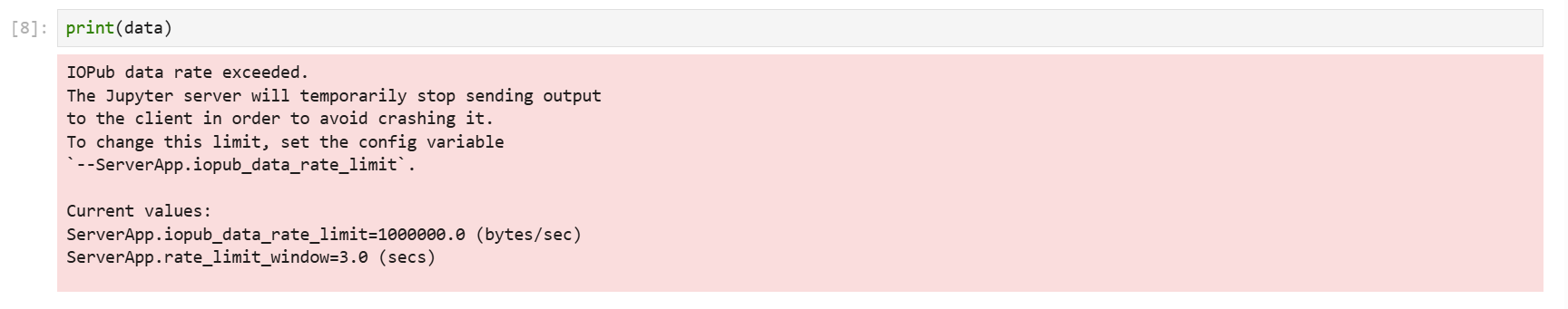
Fig. 9 Printing error for large datasets#
Working with JSON using Pandas#
Often, a better way to view and work with data is using the pandas library. The pd.json_normalize() function is useful for converting nested JSON structures into a tabular format (DataFrame).
import pandas as pd
# Normalize the JSON data into a Pandas DataFrame
# Preview the top-level json structure using `pd.json_normalize()`
# Transpose the DataFrame for an Excel-like preview
pd.json_normalize(data, errors="ignore").T
| 0 | |
|---|---|
| displayFieldName | |
| geometryType | esriGeometryPolygon |
| fields | [{'name': 'FID', 'type': 'esriFieldTypeOID', '... |
| features | [{'attributes': {'FID': 0, 'CLC_st1': '122', '... |
| fieldAliases.FID | FID |
| fieldAliases.CLC_st1 | CLC_st1 |
| fieldAliases.Biotpkt201 | Biotpkt201 |
| fieldAliases.Shape_Leng | Shape_Leng |
| fieldAliases.Shape_Area | Shape_Area |
| spatialReference.wkid | 25833 |
| spatialReference.latestWkid | 25833 |
Tabular spatial data with GeoPandas#
geopandas is an extension of pandas that adds support for geographic data. It introduces the GeoDataFrame, a data structure that can store both tabular data and geometric information.
import geopandas as gp
First, convert JSON dictionary to string:
# Ensure mydata is treated as a string path for geopandas
data_string = json.dumps(data)
# Directly reading a GeoJSON file into a GeoDataFrame
gdf = gp.read_file(data_string)
/opt/conda/envs/worker_env/lib/python3.13/site-packages/pyogrio/raw.py:198: RuntimeWarning: organizePolygons() received a polygon with more than 100 parts. The processing may be really slow.  You can skip the processing by setting METHOD=SKIP, or only make it analyze counter-clock wise parts by setting METHOD=ONLY_CCW if you can assume that the outline of holes is counter-clock wise defined
  return ogr_read(
print("\nFirst few rows of the GeoDataFrame:")
gdf.head()
First few rows of the GeoDataFrame:
| FID | CLC_st1 | Biotpkt201 | Shape_Leng | Shape_Area | geometry | |
|---|---|---|---|---|---|---|
| 0 | 0 | 122 | 5.271487 | 210.523801 | 3371.947771 | POLYGON ((415775.635 5650481.473, 415776.403 5... |
| 1 | 1 | 122 | 5.271487 | 31.935928 | 50.075513 | POLYGON ((417850.525 5650376.33, 417846.393 56... |
| 2 | 2 | 122 | 5.271487 | 810.640513 | 1543.310127 | POLYGON ((417886.917 5650544.364, 417909.326 5... |
| 3 | 3 | 122 | 5.271487 | 24.509066 | 36.443441 | POLYGON ((423453.146 5650332.06, 423453.576 56... |
| 4 | 4 | 122 | 5.271487 | 29.937138 | 40.494155 | POLYGON ((417331.434 5650889.039, 417330.611 5... |
Temporary data and ZIP files#
import zipfile
import tempfile
import requests
from pathlib import Path
sample_data_url = 'https://datashare.tu-dresden.de/s/KEL6bZMn6GegEW4/download'
A temporary directory is created to avoid downloading and storing data permanently on the local system. The file path is defined by joining the folder and the file name. For this purpose, the tempfile library, which is included with Python, is used.
# Create a temporary directory
temp = Path(tempfile.mkdtemp())
zip_path = temp / "data.zip"
Next, the requests library is used to retrieve the data from the URL, and the content is written to the temporary file.
# Download the ZIP file
response = requests.get(sample_data_url)
with open(zip_path, 'wb') as file:
    file.write(response.content)
Since the file content is in ZIP format, it must be extracted.
# Extract the contents of the ZIP file
with zipfile.ZipFile(zip_path, 'r') as zip_ref:
    zip_ref.extractall(temp)
To see the files inside the temporary folder:
Use
.glob("*")to get a generator generator listing all files.Convert the generator into a list using
list()to display the files.
# View the contents of the temp folder
print("\nContents of the temporary directory:")
list(temp.glob("*"))
Contents of the temporary directory:
[PosixPath('/tmp/tmp8pwav16r/data.zip'),
 PosixPath('/tmp/tmp8pwav16r/Biotopwert.lyr'),
 PosixPath('/tmp/tmp8pwav16r/Biotopwerte Dresden 2018 Readme .txt'),
 PosixPath('/tmp/tmp8pwav16r/Biotopwerte_Dresden_2018.gdb.zip'),
 PosixPath('/tmp/tmp8pwav16r/Biotopwerte_Dresden_2018.geojson'),
 PosixPath('/tmp/tmp8pwav16r/Biotopwert_Biodiversität.zip'),
 PosixPath('/tmp/tmp8pwav16r/clc_legend.csv'),
 PosixPath('/tmp/tmp8pwav16r/MANIFEST.TXT')]
Access a ZIP file from a remote server#
To download and extract a ZIP file from a remote server:
First, create a local working directory.
Then use a helper method
tools.get_zip_extract(), which has been prepared for this section.
from pathlib import Path

base_path = Path.cwd().parents[0]

INPUT = base_path / "00_data"
INPUT.mkdir(exist_ok=True)
Add the py module folder to your system path if necessary:
import sys

module_path = str(base_path / "py")
if module_path not in sys.path:
    sys.path.append(module_path)

from modules import tools
Use the helper function:
sample_data_url = 'https://datashare.tu-dresden.de/s/KEL6bZMn6GegEW4/download'

tools.get_zip_extract(
    uri_filename=sample_data_url,
    output_path=INPUT,
    write_intermediate=True
)
Loaded 48.03 MB of 48.04 (100%)..
Extracting zip..
Retrieved download, extracted size: 246.41 MB
Geodatabase format#
Considering a geodatabase stored as a ZIP file accessible via a URL, we must
Handle HTTP requests and ZIP files,
Create a temporary folder to avoid permanently storing data locally,
Load the geospatial data,
Work with file paths.
The following packages are used for this purpose: requests, zipfile, tempfile,geopandas and os.
import geopandas as gp
The workflow is similar to loading a locally stored geodatabase. First, the file path is generated, and the data is loaded from the defined path.
gdb_path = temp / "Biotopwerte_Dresden_2018.gdb.zip"
gdf = gp.read_file(gdb_path)
If the Geodatabase contains multiple layers, and you do not specify a layer, only one default layer will be loaded. Therefore, it is important to check which layers are available.
To do this, the listlayers() function from the Fiona library is imported:
from fiona import listlayers
Calling listlayers(gdb_path) will list the available layers in the geodatabase:
layers = listlayers(gdb_path)
print(layers)
['Biotopwerte_Dresden_2018']
Now the required layer can be explicitly loaded:
gdf = gp.read_file(gdb_path, layer="Biotopwerte_Dresden_2018")
You can quickly preview the contents of the GeoDataFrame:
gdf
Show code cell output
| CLC_st1 | Biotpkt2018 | Shape_Length | Shape_Area | geometry | |
|---|---|---|---|---|---|
| 0 | 122 | 5.271487 | 210.523801 | 3371.947771 | MULTIPOLYGON (((415775.635 5650481.473, 415776... |
| 1 | 122 | 5.271487 | 31.935928 | 50.075513 | MULTIPOLYGON (((417850.525 5650376.33, 417846.... |
| 2 | 122 | 5.271487 | 810.640513 | 1543.310127 | MULTIPOLYGON (((417886.917 5650544.364, 417909... |
| 3 | 122 | 5.271487 | 24.509066 | 36.443441 | MULTIPOLYGON (((423453.146 5650332.06, 423453.... |
| 4 | 122 | 5.271487 | 29.937138 | 40.494155 | MULTIPOLYGON (((417331.434 5650889.039, 417330... |
| ... | ... | ... | ... | ... | ... |
| 33918 | 124 | 8.000000 | 9.072443 | 4.947409 | MULTIPOLYGON (((414814.645 5666810.533, 414814... |
| 33919 | 124 | 8.000000 | 1369.670301 | 63201.087919 | MULTIPOLYGON (((414791.962 5666543.765, 414803... |
| 33920 | 124 | 8.000000 | 395.094767 | 708.068118 | MULTIPOLYGON (((415006.509 5666816.796, 415004... |
| 33921 | 231 | 10.981298 | 110.373766 | 99.282910 | MULTIPOLYGON (((417478.532 5665012.465, 417477... |
| 33922 | 231 | 10.981298 | 1401.832280 | 38939.551849 | MULTIPOLYGON (((417482.897 5665014.048, 417475... |
33923 rows × 5 columns
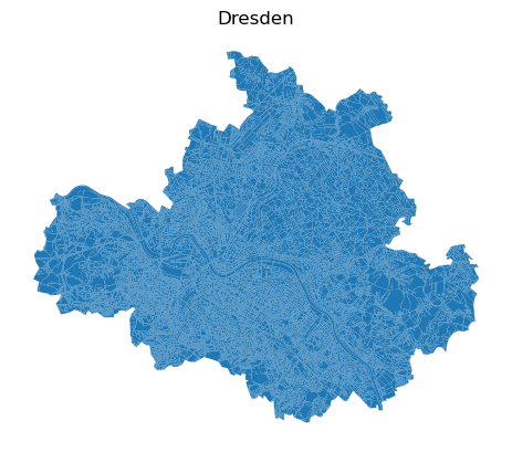
To create a simple visualization, use the plot method (explained in the Creating Map section).
Show code cell source
import matplotlib.pyplot as plt

ax = gdf.plot()
ax.set_title('Dresden')
ax.set_axis_off()
Shapefile format#
Similarly, shapefiles can be loaded and plotted using GeoPandas.
# Define the path to the shapefile
shapefile_path = INPUT / "Biotopwerte_Dresden_2018.shp"
# Read the shapefile
shapes = gp.read_file(shapefile_path)
# Preview the loaded data
shapes
Show code cell output
| CLC_st1 | Biotpkt201 | Shape_Leng | Shape_Area | geometry | |
|---|---|---|---|---|---|
| 0 | 122 | 5.271487 | 210.523801 | 3371.947771 | POLYGON ((415775.635 5650481.473, 415776.403 5... |
| 1 | 122 | 5.271487 | 31.935928 | 50.075513 | POLYGON ((417850.525 5650376.33, 417846.393 56... |
| 2 | 122 | 5.271487 | 810.640513 | 1543.310127 | POLYGON ((417886.917 5650544.364, 417909.326 5... |
| 3 | 122 | 5.271487 | 24.509066 | 36.443441 | POLYGON ((423453.146 5650332.06, 423453.576 56... |
| 4 | 122 | 5.271487 | 29.937138 | 40.494155 | POLYGON ((417331.434 5650889.039, 417330.611 5... |
| ... | ... | ... | ... | ... | ... |
| 33918 | 124 | 8.000000 | 9.072443 | 4.947409 | POLYGON ((414814.645 5666810.533, 414814.225 5... |
| 33919 | 124 | 8.000000 | 1369.670301 | 63201.087919 | POLYGON ((414791.962 5666543.765, 414803.055 5... |
| 33920 | 124 | 8.000000 | 395.094767 | 708.068118 | POLYGON ((415006.509 5666816.796, 415004.399 5... |
| 33921 | 231 | 10.981298 | 110.373766 | 99.282910 | POLYGON ((417478.532 5665012.465, 417477.463 5... |
| 33922 | 231 | 10.981298 | 1401.832280 | 38939.551849 | POLYGON ((417482.897 5665014.048, 417475.749 5... |
33923 rows × 5 columns