Spatial Overlays

Summary

Just like in GIS software, Python allows you to perform spatial overlay operations, which combine multiple spatial datasets based on their locations. In this section explores different types of spatial operations using the overlay() function in GeoPandas.

Load required libraries:

import geopandas as gp
import matplotlib.pyplot as plt
from pathlib import Path

Define file paths:

INPUT_Path = Path.cwd().parents[0] / "out"

Load input data:

input_data = gp.read_file (INPUT_Path / "clipped.shp")
ax=input_data.plot()
ax.set_axis_off() 

Check the coordinate system:

input_data.crs

Show code cell output Hide code cell output

<Projected CRS: EPSG:25833>
Name: ETRS89 / UTM zone 33N
Axis Info [cartesian]:
- E[east]: Easting (metre)
- N[north]: Northing (metre)
Area of Use:
- name: Europe between 12°E and 18°E: Austria; Croatia; Denmark - offshore and offshore; Germany - onshore and offshore; Italy - onshore and offshore; Norway including Svalbard - onshore and offshore.
- bounds: (12.0, 34.79, 18.01, 84.01)
Coordinate Operation:
- name: UTM zone 33N
- method: Transverse Mercator
Datum: European Terrestrial Reference System 1989 ensemble
- Ellipsoid: GRS 1980
- Prime Meridian: Greenwich

Load overlay data:

Show code cell source Hide code cell source

# District data from the Dresden portal Already mentioned in the Clipping Data chapter
import requests
geojson_url = "https://kommisdd.dresden.de/net4/public/ogcapi/collections/L137/items"
response = requests.get(geojson_url)
if response.status_code == 200:
    gdf = gp.read_file(geojson_url)
    
else:
    print("Error:", response.text)

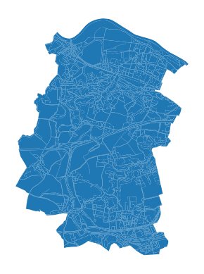
overlay_data= gdf[gdf['id']== '99']
ax=overlay_data.plot()
ax.set_axis_off()

Check the coordinate system:

overlay_data.crs

Show code cell output Hide code cell output

<Geographic 2D CRS: EPSG:4326>
Name: WGS 84
Axis Info [ellipsoidal]:
- Lat[north]: Geodetic latitude (degree)
- Lon[east]: Geodetic longitude (degree)
Area of Use:
- name: World.
- bounds: (-180.0, -90.0, 180.0, 90.0)
Datum: World Geodetic System 1984 ensemble
- Ellipsoid: WGS 84
- Prime Meridian: Greenwich

In case the coordinate system of the layers are different match the coordinates using to_crs method.

overlay_data = overlay_data.to_crs(input_data.crs)

The overlay() function in GeoPandas allows different types of spatial operations, defined by the how parameter.

The following list explains available operations:

• intersection – Returns the overlapping (shared) area between two geometries.

• union - Merges both geometries into a single geometry.

• difference - Subtract second geometry from the first geometry.

• symmetric_difference - The areas that are in either of the two geometries, but not in both

• identity- Keeps the shape of the first geometry while adding overlapping parts from the second geometry.

Overlay Analysis

For more information, check the GeoPandas spatial overlay documentation.

Examples how to apply these operations:

# Intersection: Find the overlapping (shared) area between input_data and overlay_data
out_intersection = gp.overlay(
    input_data, overlay_data,
    how='intersection')

# Union: Merge input_data and overlay_data into one geometry
out_union = gp.overlay(
    input_data, overlay_data,
    how='union')

# Difference: Subtract overlay_data from input_data
out_difference = gp.overlay(
    input_data, overlay_data,
    how='difference')

# Symmetric Difference: Get areas that are in either geometry, but not both
out_symmetric = gp.overlay(
    input_data, overlay_data,
    how='symmetric_difference')

# Identity: Retain the first geometry but mark overlapping areas with the second geometry
out_identity = gp.overlay(
    input_data, overlay_data,
    how='identity')

/tmp/ipykernel_2565/1074488158.py:7: UserWarning: `keep_geom_type=True` in overlay resulted in 42 dropped geometries of different geometry types than df1 has. Set `keep_geom_type=False` to retain all geometries
  out_union = gp.overlay(
/tmp/ipykernel_2565/1074488158.py:17: UserWarning: `keep_geom_type=True` in overlay resulted in 42 dropped geometries of different geometry types than df1 has. Set `keep_geom_type=False` to retain all geometries
  out_symmetric = gp.overlay(

The results can be inspected by using the print function, which will show the first few rows of the overlayed dataset.

Example:

print(out_symmetric.head())

  CLC_st1  Biotpkt201   Shape_Leng     Shape_Area   id  bez bez_lang  \
0     112    7.150000   122.271774     457.162617  NaN  NaN      NaN   
1     311   16.503069   315.595049    3746.157997  NaN  NaN      NaN   
2     211    6.336151  2119.697191  138157.775431  NaN  NaN      NaN   
3     211    6.336151  1130.132105   60835.673105  NaN  NaN      NaN   
4     324   14.000424   435.445295    4721.684346  NaN  NaN      NaN   

   flaeche_km2  sst sst_klar historie aend  \
0          NaN  NaN      NaN      NaN  NaN   
1          NaN  NaN      NaN      NaN  NaN   
2          NaN  NaN      NaN      NaN  NaN   
3          NaN  NaN      NaN      NaN  NaN   
4          NaN  NaN      NaN      NaN  NaN   

                                            geometry  
0  POLYGON ((404140.322 5654373.512, 404139.007 5...  
1  POLYGON ((403977.642 5654356.446, 403988.445 5...  
2  POLYGON ((405646.102 5654518.48, 405646.102 56...  
3  MULTIPOLYGON (((402546.984 5654396.33, 402546....  
4  POLYGON ((402599.505 5654413.851, 402593.69 56...  

The results can be visualized by using the plot function.

Example:

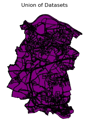
ax = out_union.plot(
    color="purple", 
    edgecolor="black")
ax.set_title("Union of Datasets")
ax.set_axis_off()

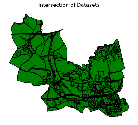
ax = out_intersection.plot(
    color="green", 
    edgecolor="black")
ax.set_title("Intersection of Datasets")
ax.set_axis_off()

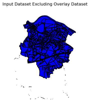
ax = out_difference.plot(
    color="blue", 
    edgecolor="black")
ax.set_title("Input Dataset Excluding Overlay Dataset")
ax.set_axis_off()