Setup & Getting familiar with Jupyter#
Summary
This chapter provides a brief introduction to the key components of the Jupyter. For a more detailed information, please see jupyter.org.
Jupyter is a software that includes various tools for interactive computing. These training materials are built using Jupyter Notebooks, which are interactive documents that combine explanations, code, and outputs in one place. The notebooks were created using JupyterLab, which is a web-based development environment that provides an integrated workspace for notebooks, text editors, terminals, and more. To make navigation easier, individual notebooks have been structured into a Jupyter Book, which organizes the content into chapters and pages.
Learn more about Jupyter Notebook, JupyterLab and Jupyter Book.
How to use the Notebooks?#
The notebooks can be used in several ways:
As a source of information: Use the notebooks as a source of information by reading the main chapters and skipping sections that involve Python specifics.
For code snippets: Browse through the chapters and select and copy relevant code snippets to use in your own projects.
Interactively: Run the Jupyter Notebooks to explore and experiment with the workflows, trying out the code and modifying it for your needs.
How to copy code snippets?#
The page is organized into sections called ‘cells,’ which may include text explanations, images, or code.
To copy a code snippet, click the copy icon in the top-right corner of the code cell.
# See the copy button on the right corner when you hover over this text.
Tip
In Jupyter Notebooks, text cells use Markdown, a simple markup language for formatting notes, documents, presentations, and websites. Markdown works across all operating systems and is converted to HTML for display in web browsers.
Learn more about using Markdown.
How to run the training materials interactively?#
In Python, “dependencies” typically refer to packages and libraries that the code needs to work properly. Packages and libraries are collections of pre-written code that help you perform various tasks more easily. Each package or library is designed for a specific purpose, such as visualising data.
To successfully run the workflows in these notebooks, you must have the required packages or libraries installed. The first software that is needed is JupyterLab.
Not familiar with Python packages or libraries?
The Python Standard Library Documentation and the lists below provide selected standard library modules as well as third-party packages and libraries.
Selected standard library modules (pre-installed with Python)
Selected third-party packages and libaries (require installation)
requests: Simplifies making HTTP requests, allowing users to easily send and receive data from web APIs
shapely: Geometric operations and spatial queries
numpy: Numerical computing and array operations
holoviews: High-level data visualization framework
geoviews: Geographic data visualizations for HoloViews
geopandas: Geospatial data manipulation using pandas.
pyproj: Cartographic projections and coordinate transformations library
cartopy: Drawing maps for data analysis and visualisation
bokeh: Interactive web-based visualizations with JavaScript integration.
matplotlib: Plotting and data visualization library
ggplot2: System for declaratively creating graphics
Installing JupyterLab is relatively easy:
pip install jupyterlab
jupyter lab # run jupyterlab
However, from there, Python package management, version conflicts, dependency issues and many other challenges can make it very difficult for beginnings to reproduce the outputs we show here. You have different options that we explain below.
Jupyter4NFDI#
You can interactively run this notebook on the Jupyter4NFDI platform using Binder integration. Simply click the Binder icon in the upper-right corner of the page.

Fig. 1 Run a notebook in this book via the Jupyter4NFDI platform using Binder integration.#
🔐 Authentication via Helmholtz AAI#
Jupyter4NFDI utilizes the Helmholtz Authentication and Authorization Infrastructure (AAI) for secure access. This federated login system allows you to authenticate using your institutional credentials or social identities like GitHub, Google, or ORCID.
Click the Binder icon: Located in the top-right corner of the notebook page.
Select your Identity Provider (IdP): Choose your home institution or preferred social IdP from the list.
Authenticate: Enter your credentials as prompted.
Access the notebook: After successful authentication, you’ll be directed to an interactive Jupyter environment with the notebook ready to use.
Tip for IOER Members.
If you’re affiliated with the IOER, select TU Dresden as your Identity Provider during the login process.
For a list of connected organizations supporting eduGAIN, refer to the Helmholtz AAI documentation.
Additional Resources:
Jupyter4NFDI Hub: https://hub.nfdi-jupyter.de/hub/home
Jupyter4NFDI Documentation: https://jupyterjsc.pages.jsc.fz-juelich.de/docs/jupyter4nfdi/
Potential dependendy conflicts ahead.
The tradeoff here is that you must install all dependencies before running notebooks. We include a script at the start of notebooks, but the Python ecosystem is always evolving and some dependency conflicts may arise at some point. See below for an alternative solution that guarantees full reproducibility.
Carto-Lab Docker#
To ensure full reproducibility of the training materials, we use a prepared system environment called Carto-Lab Docker.
Carto-Lab Docker includes
Jupyter Lab
A Python environment with major cartographic packages pre-installed
The base system (Linux)
All these components are packaged in a Docker container, which is versioned and made available through a registry. The version number allows you to pull the correct archive container to run these notebooks. Below we show the version of Carto-Lab Docker used:
Last updated: Sep-22-2025, Carto-Lab Docker Version 1.0.1
See the Carto-Lab Docker docs for installation instructions
This is from the Carto-Lab Docker docs.
# create a shallow clone (no git history, just the latest files)
git clone --depth 1 https://gitlab.vgiscience.de/lbsn/tools/jupyterlab.git
cd jupyterlab
cp .env.example .env
nano .env
# Enter the Carto-Lab Docker version you want to use
# TAG=v0.26.1
docker network create lbsn-network
docker-compose pull && docker-compose up -d
We only guarantee reproducibility with Carto-Lab Docker
Due to the wide variety of possible setups, operating systems (Windows, Linux, Mac), software versions and changing environments, we can only guarantee complete reproducibility with the exact Carto-Lab Docker version shown above. You may still be lucky if you use some of the alternatives we show you below.
In general, we recommend to avoid Windows under any circumstances. If you are working in Windows, a better alternative is either to use Windows Subsystem for Linux (WSL) or to run these notebooks in the cloud somewhere (ask your IT/Admin). For instance, Carto-Lab Docker can also be run in the cloud.
Clone the training materials#
In order to use the training materials, the repository must be cloned. Open a terminal and type the following command:
# create a shallow clone (no git history, just the latest files)
git clone --depth 1 https://gitlab.hrz.tu-chemnitz.de/ioer/fdz/jupyter-book-nfdi4biodiversity.git
Use the Jupyter Terminal
You can use the terminal that is provided by Jupyter. At your Jupyter Dashboard, click the following Icon:
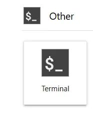
Fig. 2 This is the terminal icon.#
Afterwards, type:
cd /home/jovyan/work/
# create a shallow clone (no git history, just the latest files)
git clone --depth 1 https://gitlab.hrz.tu-chemnitz.de/ioer/fdz/jupyter-book-nfdi4biodiversity.git
/home/jovyan/work/is the path to the default home folder in Jupyter. The home folder is the folder you see in the explorer on the left side when you are logged in to Jupyter.
Jupyterlab: Basic key commands#
After these steps, you are ready to go. You can find the individual notebooks of the training materials in the subfolder notebooks/.
These are the most important key commands, to get you started.
SHIFT + ENTER → Run the current cell and go to the next
CTRL + ENTER → Run multiple selected cells
CTRL + X → Cut selected cells
d d (press d twice) → Delete selected cells
Installing dependencies individually#
You can also install the packages individually:
Install all packages for all notebooks in a single environment (harder, but less work)
or install all packages for each notebook into a separate environment (easier, but more work)
For Option 1, you can start with the environment.yml from Carto-Lab Docker and install the environment manually with:
conda env create -f environment.yaml
Afterwards, you must install jupyterlab into the above environment manually with:
conda activate worker_env
conda install -c conda-forge jupyterlab
For Option 2, we we provide a summary of the packages used and the specific versions at the end of each notebook chapter,
Example:
List of package versions used in this notebook
| package | python | python | dask | pandas | datashader | matplotlib | geopandas |
|---|---|---|---|---|---|---|---|
| version | 3.9.23 | Not installed | 2024.8.0 | 2.3.1 | 0.16.3 | 3.9.4 | 1.0.1 |
To install the above packages, use e.g.:
pip install python==3.11.6 dask==2024.12.1 datashader==0.17.0 geopandas==0.14.4 matplotlib==3.10.1 pandas==2.2.3
If you see an error above, try the below instructions for “Temporary package installs” and run the cell above again.
Temporary package installs#
Sometimes, a default environment exists that already includes many packages. Only some new packages need to be installed for certain notebooks. In these cases, it can be Ok to install packages temporarily directly from within Jupyter.
Example notebook
We do this, for example, for owslib in our workflow in Data Retrieval: IOER Monitor: The Carto-Lab Docker environment does not contain this package and we only need it once to query the IOER Monitor API.
You can install packages temporarily by issuing bash commands directly in a code cell with a !-prefix.
!pip install owslib
We have written a little helper script that comes with the training materials that also checks if the package is already installed. Run the cell below, then execute the cell above (List package versions) again and observe the changes.
import sys
pyexec = sys.executable
print(f"Current Kernel {pyexec}")
!../py/modules/pkginstall.sh "{pyexec}" myst-nb owslib geopandas geoviews holoviews matplotlib shapely cartopy contextily mapclassify adjustText
Current Kernel /opt/conda/envs/worker_env/bin/python3.9
Installing myst-nb...
WARNING: Running pip as the 'root' user can result in broken permissions and conflicting behaviour with the system package manager, possibly rendering your system unusable. It is recommended to use a virtual environment instead: https://pip.pypa.io/warnings/venv. Use the --root-user-action option if you know what you are doing and want to suppress this warning.
Installed myst-nb 1.3.0.
Installing owslib...
WARNING: Running pip as the 'root' user can result in broken permissions and conflicting behaviour with the system package manager, possibly rendering your system unusable. It is recommended to use a virtual environment instead: https://pip.pypa.io/warnings/venv. Use the --root-user-action option if you know what you are doing and want to suppress this warning.
Installed owslib 0.31.0.
geopandas already installed (version 1.0.1).
geoviews already installed (version 1.12.0).
holoviews already installed (version 1.20.2).
matplotlib already installed (version 3.9.4).
shapely already installed (version 2.0.7).
cartopy already installed (version 0.23.0).
contextily already installed (version 1.6.2).
mapclassify already installed (version 2.8.1).
adjustText already installed (version 1.3.0).
Have a look at pkginstall.sh
#!/bin/bash

################################################################################
#
# Environment-agnostic Python package installer.
# - Use the Python binary passed as first argument
# - Check if each package is available; install it if not
#
################################################################################

set -e
set -u

PYTHON_BIN="$1"
shift  # Shift arguments so $@ now contains only packages

pkgs=( "$@" )

for pkg in "${pkgs[@]}"; do
    import_name="${pkg//-/_}"
    if "$PYTHON_BIN" -c "import ${import_name}" 2>/dev/null; then
        version=$("$PYTHON_BIN" -c "import ${import_name}; print(getattr(${import_name}, '__version__', 'unknown'))")
        echo "${pkg} already installed (version ${version})."
    else
        echo "Installing ${pkg}..."
        "$PYTHON_BIN" -m pip install "$pkg" --quiet
        if "$PYTHON_BIN" -c "import ${import_name}" 2>/dev/null; then
            version=$("$PYTHON_BIN" -c "import ${import_name}; print(getattr(${import_name}, '__version__', 'unknown'))")
            echo "Installed ${pkg} ${version}."
        else
            echo "Warning: ${pkg} installed but version could not be determined."
        fi
    fi
done
Note
This script should work in most environments. Make sure you specify the name of the current kernel environment, e.g:
import sys
pyexec = sys.executable
print(f"Current Kernel {pyexec}")
!../py/modules/pkginstall.sh "{pyexec}" geopandas
How to import Packages and Libraries#
After successfully installing the package, you need to import it in your notebook to be able to use their functions.
Create a new code cell where you can write your statements. To import a package, use the “import” keyword followed by the “package name”.
Example: import pandas
Or to make it easier to call during coding use an alias :
Example: import pandas as pd

This cell is not showing any output unless the package or library not installed successfully :
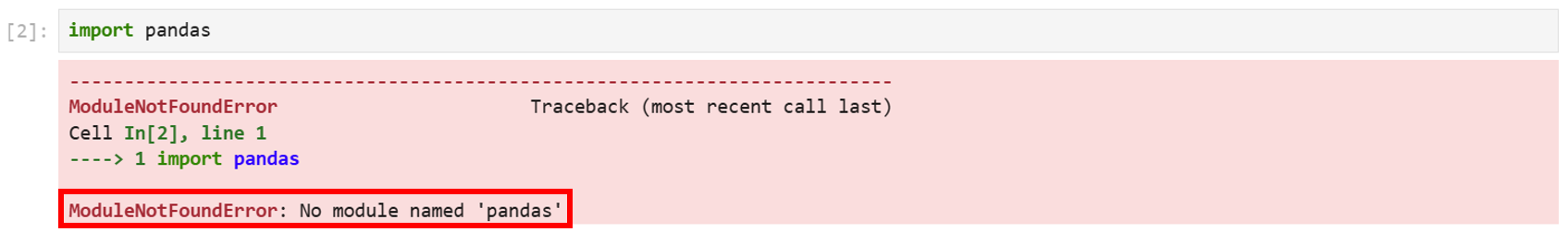
If the installation was successful but still the issue persists, it could be due to using the wrong environment or kernel.
Wrong Environment: Package or Library is not installed in the current environment:
Solution: Activate the correct environment, then restart Jupyter.
Wrong Kernel: Package or Library is not installed in the selected Jupyter kernel.
Solution: Switch to the correct kernel via the upper-right menu in Jupyter.
