Buffering Data

Buffering Data#

In some analysis it is necessary to find the influence of a feature in the surrounding areas, in this situation the buffer operation will help.

To create buffers, first add the geopandas package.

from pathlib import Path
import geopandas as gp
import matplotlib.pyplot as plt
import matplotlib.patches as mpatches

base_path = Path.cwd().parents[0]
INPUT = base_path / "00_data"
OUTPUT = base_path / "out"

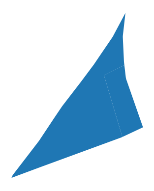
The input data is then loaded:

input_data = gp.read_file(OUTPUT / "clipped.shp")[58:60]
ax=input_data.plot()
ax.set_axis_off() 

../_images/4cefa114bb47c51d1b7f2264f1624d819f0f7cba53673eb10bfd7381bd5fd171.png

buffer_data = input_data.copy()

Non-Dissolved Buffers#

Using the buffer method, buffers are created by modifying the geometry of the input data. The value defined within the buffer method is the size of the buffer and its unit depends on the coordinate system of the data.

Example of Units

WGS 84 (EPSG Code:4326): Degrees.
ETRS89 / UTM Zone 32N (EPSG Code:25832): Meters.

buffer_data['geometry'] = buffer_data['geometry'].buffer(8)

The original data and the result of the buffer is visualized using the parameters in the plot function:

ax: Overlays multiple plots on a map.
alpha: Controls the transparency of the datasets for better visualization. (ranges from 1 to 0 (fully transparent))

../_images/16.png — Fig. 16 Color transparency from 0 (fully transparent) to 1 (completely visible)#

Also, the Patch function in matplotlib, creates a colored patch that can be used as a legend entry in a plot.

color: sets the color of the patch
label: specifies the lable of that color in the legend

Then legend function in Matplotlib adds the legend to a plot.

handles: list of objects in the legend
loc: specifies the location of the legend within the plot (lower left/right, upper left/right, center, lower/upper center)

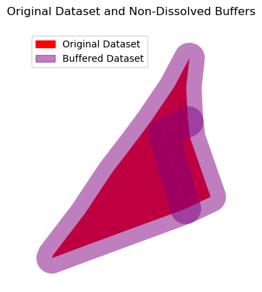
ax = input_data.plot(color='red', alpha=1)
buffer_data.plot(ax=ax, color='purple', alpha=0.5)

input_patch = mpatches.Patch(color='red', label='Original Dataset')
buffer_patch = mpatches.Patch(color='purple', alpha=0.5, label='Buffered Dataset')

ax.legend(handles=[input_patch, buffer_patch], loc='upper left')

ax.set_title("Original Dataset and Non-Dissolved Buffers")
ax.set_axis_off()

../_images/71b8a8ace8711c9a881f73c29cd21aee047d464e818b44a1c689c4c170f152af.png

The geometry column can be checked both before and after the buffer operation to observe the changes.

input_data.head(3)

Show code cell output Hide code cell output

	CLC_st1	Biotpkt201	Shape_Leng	Shape_Area	geometry
58	112	5.000000	109.892100	542.707900	POLYGON ((405111.872 5654588.962, 405124.639 5...
59	311	16.503069	288.028174	2249.972297	POLYGON ((405111.872 5654588.962, 405123.395 5...

buffer_data.head(3)

Show code cell output Hide code cell output

	CLC_st1	Biotpkt201	Shape_Leng	Shape_Area	geometry
58	112	5.000000	109.892100	542.707900	POLYGON ((405104.204 5654586.681, 405104.015 5...
59	311	16.503069	288.028174	2249.972297	POLYGON ((405064.569 5654552.423, 405073.941 5...

Dissolved Buffers#

When the datasets are printed after buffer operation, the number of features remains the same. This indicates the buffer operation creates an individual buffer for each feature, rather than merging overlapping areas.

input_data.shape

(2, 5)

buffer_data.shape

(2, 5)

The dissolve function can merge all the buffers at once, creates a single feature from the whole dataset:

dissolved_buffer = buffer_data.dissolve()
dissolved_buffer

	geometry	CLC_st1	Biotpkt201	Shape_Leng	Shape_Area
0	POLYGON ((405133.453 5654588.899, 405133.462 5...	112	5.0	109.8921	542.7079

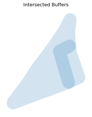
If only the merging of intersected buffers is required, the overlapping areas need to be identified first.

This can be done by overlaying the dataset with itself to find the areas where the buffers intersect:

intersected_buffers = gp.sjoin(
    buffer_data, 
    buffer_data[['CLC_st1','geometry']], 
    how="inner", 
    predicate="intersects")
intersected_buffers.head(5)

Show code cell output Hide code cell output

	CLC_st1_left	Biotpkt201	Shape_Leng	Shape_Area	geometry	index_right	CLC_st1_right
58	112	5.000000	109.892100	542.707900	POLYGON ((405104.204 5654586.681, 405104.015 5...	58	112
58	112	5.000000	109.892100	542.707900	POLYGON ((405104.204 5654586.681, 405104.015 5...	59	311
59	311	16.503069	288.028174	2249.972297	POLYGON ((405064.569 5654552.423, 405073.941 5...	58	112
59	311	16.503069	288.028174	2249.972297	POLYGON ((405064.569 5654552.423, 405073.941 5...	59	311

ax = intersected_buffers.plot(alpha= 0.1)
ax.set_title("Intersected Buffers")
ax.set_axis_off()

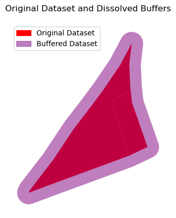
../_images/60d0a67ab5e4644fbcbf4c80f608b3680a0f4fb0b295fc4b1eb40146b84d8af9.png

Then the dissolve operation is performed to merge only the intersected buffers.

dissolving_buffer = intersected_buffers.dissolve()
dissolving_buffer

	geometry	CLC_st1_left	Biotpkt201	Shape_Leng	Shape_Area	index_right	CLC_st1_right
0	POLYGON ((405133.453 5654588.899, 405133.462 5...	112	5.0	109.8921	542.7079	58	112

ax = dissolving_buffer.plot(alpha= 0.1)
ax.set_title('Dissolved Buffers')
ax.set_axis_off()

../_images/10d8dbe01719e9aab895b0387bfffaeacb030d64d608f08a0fcc2d7fd37e196d.png

ax = input_data.plot(color='red', alpha=1)
dissolving_buffer.plot(ax=ax, color='purple', alpha=0.5)

input_patch = mpatches.Patch(color='red', label='Original Dataset')
buffer_patch = mpatches.Patch(color='purple', alpha=0.5, label='Buffered Dataset')

ax.legend(handles=[input_patch, buffer_patch], loc='upper left')

ax.set_title("Original Dataset and Dissolved Buffers")
ax.set_axis_off()

../_images/d386c097f6565c48ab3d0a05c3a392679c520eace570db66aaba5fb5f0647018.png

Comparison

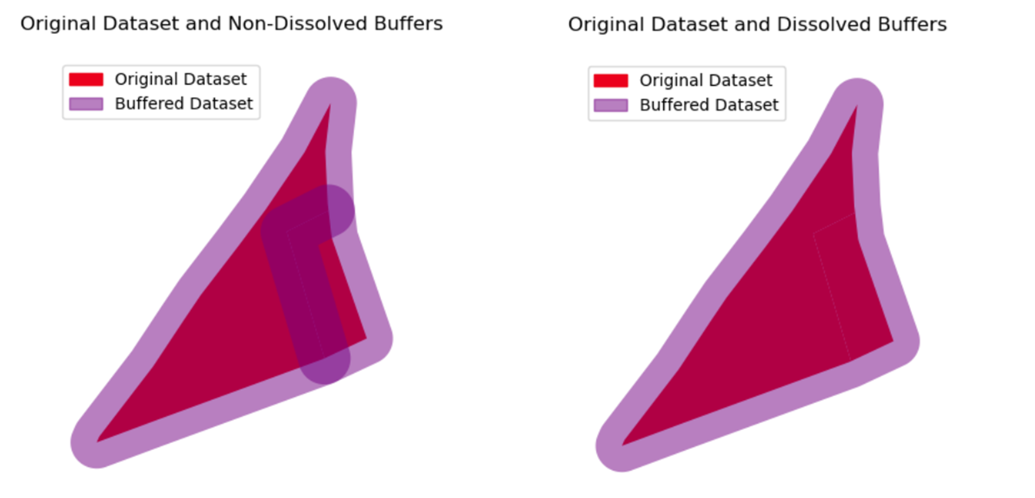
../_images/18.png — Fig. 17 Non-Dissolved Buffers VS Dissolved Buffers#

Buffer Parameters

In addition to the distance parameter, which indicates the size of the buffer, there are other parameters that help in processing and visualizing the output.

resolution is a parameter that defines the number of segments used to create a quarter circle. The larger values for this parameter cause slower processing.

cap_styledefines the shape of the end of the buffer, which is mostly used for line features.

cap_style = 1 defines Round shape.
cap_style = 2 defines Flat shape.
cap_style = 3 defines Square shape.

join_style defines the shape of the corner and edges in the buffers.

join_style = 1 defines Round shape.
join_style = 2 defines Mitre shape.
join_style = 3 defines Bevel shape.

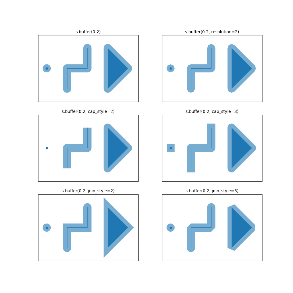
https://geopandas.org/en/stable/_images/buffer.png — Fig. 18 Visualization of Buffer Parameters (Source: GeoPandas website).#

input_data = gp.read_file(OUTPUT / "clipped.shp")[127:128]
buffer_data = input_data.copy()

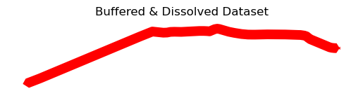
The following code creates a buffer of:

20 (The unit depends on the CRS),
with a resolution of 8,
round ends,
and beveled corners.

buffer_data['geometry'] = input_data['geometry'].buffer(
    distance=20, 
    resolution=8, 
    cap_style=2, 
    join_style=3)

ax = buffer_data.plot(color='red')
ax.set_title("Buffered & Dissolved Dataset")
ax.set_axis_off()

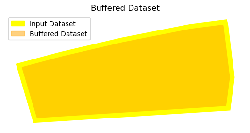
../_images/0e989886e3c86d9b828f8ff70c9a571983c497cda0a55899efb187c9e6df5148.png

Negative Buffers#

Sometimes a feature is so large that it affects the analysis. In such cases, a negative buffer is defined to reduce the impact of the feature itself.

The desired feature or dataset is loaded first.

First_data = gp.read_file(OUTPUT / "clipped.shp")[2:3]
copy_data = First_data.copy()

In this case, simply define a negative value for the distance parameter, instead of a positive value.

copy_data['geometry'] = copy_data['geometry'].buffer(distance= -4) 

ax = First_data.plot(color='yellow', alpha=1)
copy_data.plot(ax=ax, color='orange', alpha=0.5)

input_patch = mpatches.Patch(color='yellow', label='Input Dataset')
buffer_patch = mpatches.Patch(color='orange', alpha=0.5, label='Buffered Dataset')

ax.legend(handles=[input_patch, buffer_patch], loc='upper left')

ax.set_title("Buffered Dataset")
ax.set_axis_off()

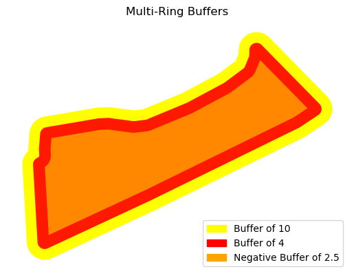
../_images/2d0854c07a22abe4ba4e439cfd943550ea9828893101765bc173be48811751e1.png

Multi-Ring Buffers#

To analyze the effect of a feature at different distances, it can be helpful to create concentric buffer zones (multi-ring buffers) around the feature.

As these buffers needed to combine the pandas library should be imported.

import pandas as pd

The data is loaded.

First_data = gp.read_file(OUTPUT / "clipped.shp")[11:12]
copied_data = First_data.copy()

The buffer distances are defined as a list.

distances = [ -2.5, 4, 10] 

An empty list is created for containing the buffers for the defined distances.

buffer_data = []

A for loop is used to generate buffers around each feature in the dataset.

Then both the distances and the geometry of buffers store in the empty list that already created.

for items in distances:
    buffered_geom = copied_data.geometry.buffer(items)
    for geom in buffered_geom:
        buffer_data.append({'geometry': geom, 'distance': items})

Then the list converts to a GeoDataFrame.

buffers = gp.GeoDataFrame(buffer_data)

print (buffers)

                                            geometry  distance
POLYGON ((404964.703 5654242.885, 404964.965 5...      -2.5
POLYGON ((404960.805 5654248.128, 404960.88 56...       4.0
POLYGON ((404955.439 5654251.784, 404955.414 5...      10.0

All the buffers can then be plotted together in the same window:

First, a separate dataset is created for each buffer distance by selecting the corresponding distance variable.

buffers_2 = buffers[buffers['distance'] == -2.5]
buffers_4 = buffers[buffers['distance'] == 4]
buffers_10 = buffers[buffers['distance'] == 10]

Then as already mentioned in this section, using the ax parameter the datasets overlay for visualization.

ax = buffers_10.plot(color='yellow', label='Buffer of 10')
buffers_4.plot(ax=ax, color='red', alpha= 0.9,label='Buffer of 4')
buffers_2.plot(ax=ax, color='orange', alpha= 0.8,label='Negative Buffer of 2.5')

#legend
legend_handles = [
    mpatches.Patch(color='yellow', label='Buffer of 10'),
    mpatches.Patch(color='red', label='Buffer of 4'),
    mpatches.Patch(color='orange', label='Negative Buffer of 2.5')

]
ax.set_axis_off()  
plt.title("Multi-Ring Buffers")
plt.legend(handles=legend_handles, loc='lower right')
plt.show()

../_images/e6b6f283b6433ef6805cd84238a42b1fc33de9dfd971ddd1f8483cb0426be7ab.png

Also to be able to compare the created buffers for each feature, radio button can be helpful.

For this reason, the ipywidgets library and interactive function added allow the creation of an interactive widget for comparing.

import ipywidgets as w
from ipywidgets import interactive

The RadioButtons function then used to create the radio buttons for the user to select from.

value: Default selected value
options: Options for radio buttons
description: Title for the button lists

radiobutton = w.RadioButtons(
    value= -2.5,                    
    options=[10, 4, -2.5],       
    description="Buffer Distance",
)

Then, a function is defined that plots the selected buffer data based on the button selected in the radio buttons.

Then, using the interactive function, the function and the widget are linked.

interactive(function_name, parameter1=widget1, parameter2=widget2, …)

ex: interactive_plot = interactive(plot_data, radiobutton= radiobutton)

first radiobutton: parameter which has been called in the plot_data function
second radiobutton: radiobutton widget that already created to select

def plot_data(radiobutton):
    fig, ax = plt.subplots()

    copied_data.plot(ax=ax, edgecolor='black', facecolor='none', linewidth=2, alpha=1)

    if radiobutton == 10:
        buffers_10.plot(ax=ax, color='red', alpha=0.5)
    elif radiobutton == 4:
        buffers_4.plot(ax=ax, color='yellow', alpha=0.5)
    elif radiobutton == -2.5:
        buffers_2.plot(ax=ax, color='orange', alpha=0.5)

    legend_handles = [
    mpatches.Patch(edgecolor='black', facecolor='none', label='Original Layer'),
    mpatches.Patch(color='red', label='Buffer of 10'),
    mpatches.Patch(color='yellow', label='Buffer of 4'),
    mpatches.Patch(color='orange', label='Negative Buffer of 2.5')]
    plt.legend(handles=legend_handles, loc= 'upper left')

    ax.set_title("Original Layer with Buffers")
    ax.set_axis_off()

    plt.show()

interactive_plot = interactive(plot_data, radiobutton= radiobutton)

display(interactive_plot)

Interactive Visualization

Buffering Data

Contents

Buffering Data#

Non-Dissolved Buffers#

Dissolved Buffers#

Negative Buffers#

Multi-Ring Buffers#