Publishing

Publishing#

Publishing your results can mean several things:

Writing a manuscript and submitting the results to a journal for (double-blind) peer review.
Creating a data publication, ideally submitted with your text manuscript, for data transparency & reproducibility.
Publish your git repository, making it available for others to find and read your notebooks.

We provide a short step-by-step guide on how to publish Jupyter notebooks together with the generated visuals and output as a data publication.

Make a release version#

When you are finished with your work, e.g. before submitting your manuscript for the first round of review, create a git release for your notebook repository and give it a version number:

git tag -a v1.0.0 -m "Major release before submitting to Journal"
git push --tags

Hint

This adds a marker to your Git repository that can be easily found and referenced at any later stage. If you submit a minor or major revision at a later date, add another version tag to describe your progress.

After pushing your tag to Github or Gitlab, you can (and should!) create a Release from it, where you can attach data and other output information. Releases can be cited with (e.g.) Zenodo or ioerDATA.

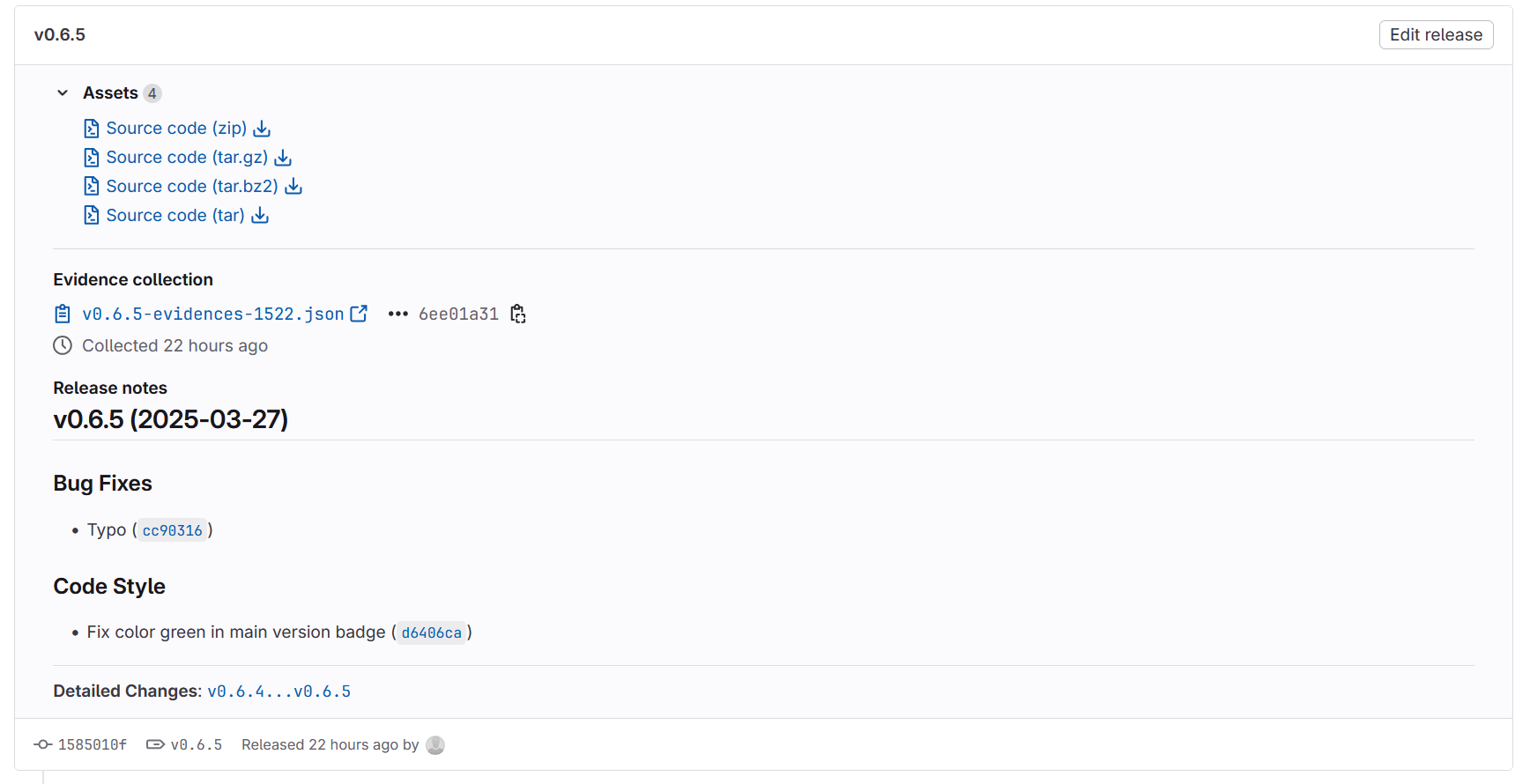
../_images/release.png — Fig. 7 A release from our Gitlab repository based on the version `v0.6.5`-tag of the training materials.#

Create HTML versions of all your notebooks#

This is an optional step, but recommended because reviewers may not have Jupyter Lab to open your *.ipynb notebooks. By converting notebooks to HTML format, you can archive any code together with the generated visuals. You can convert notebooks directly in Jupyter with the below command.

!jupyter nbconvert --to html \
    --output-dir=../out/ ./205_publish.ipynb \
    --template=../nbconvert.tpl \
    --ExtractOutputPreprocessor.enabled=False

[NbConvertApp] Converting notebook ./205_publish.ipynb to html
[NbConvertApp] Writing 348507 bytes to ../out/205_publish.html

Hint

If you are using Carto-Lab Docker, replace html with html_toc in the above cell. This will automatically add a Terms of Content to the sidebar of your HTML, based on the headers (Markdown) in your Jupyter notebook.

Add conversion command at the end of every notebook

It is a good idea to add this command to every notebook, so it is run after every notebook change.

Attach the static HTML files as Supplementary Material for your submitted paper

These HTML versions of the notebooks are ideal for attaching directly to your publications when submitting a manuscript as Supplementary Materials (SM). They are like a portable archive version that contains your documentation, code and output graphics at the time of publication. This is the most important information and should be attached directly to your paper. This also helps reviewers to have a look at your workflow if they do not want to run the notebooks themselves.

In addition to these HTML files, the original notebook files (*.ipynb) and accompanying data should be made available in a proper data publication, which we show below.

Create a ZIP file with all your output data#

Once you have exported all notebook HTMLs and figures, create a ZIP archive that includes all your data, notebooks, HTML files, and figures. You can create this ZIP file directly in Jupyter, based on the latest Git version we created earlier.

Remove any previous releases

!rm ../out/*.zip

This Bash command cleans up any previous ZIP files in the out/ directory. The ! indicates it’s a shell command, not Python.

See an error?

The error rm: cannot remove ‘../out/*.zip’: No such file or directory indicates that there are no zip files in the directory that can be deleted. This is expected if you run this notebook for the first time.

Prepare a release

Make sure that 7z is available. Carto-Lab Docker comes with 7z. If you are using this in a rootfull container, you can use !apt install p7zip-full. Otherwise (e.g. in Jupyter4NFDI Hub), we must retrieve the binary below.

%%bash
# Check if '7z' is already available globally or in ~/bin
if ! command -v 7z >/dev/null 2>&1 && [ ! -x "$HOME/bin/7z" ]; then
  echo "7z not found. Installing local copy..."
  mkdir -p ~/bin && cd ~/bin
  wget -q https://www.7-zip.org/a/7z2301-linux-x64.tar.xz
  tar -xf 7z2301-linux-x64.tar.xz
  ln -sf ~/bin/7zz ~/bin/7z
else
  echo "7z is already available."
fi

7z is already available.

Create a new release *.zip file

We want to create a ZIP file with the current release version in the name. We can get this with the following command:

!git describe --tags --abbrev=0

v1.8.0

Create the release file:

%%bash
export PATH="$HOME/bin:$PATH" \
    && cd .. && git config --local --add safe.directory '*' \
    && RELEASE_VERSION=$(git describe --tags --abbrev=0) \
    && 7z a -tzip -mx=9 out/release_$RELEASE_VERSION.zip \
    py/* out/* resources/* tmp/* *.bib notebooks/*.ipynb 00_data/* \
    *.md *.yml *.ipynb nbconvert.tpl conf.json pyproject.toml \
    -x!py/__pycache__ -x!py/modules/__pycache__ -x!py/modules/.ipynb_checkpoints \
    -y > /dev/null

Attach the static HTML files as Supplementary Material for your submitted paper

This may take a while. If you want to see output from the 7z process, remove -y > /dev/null (and the preceeding backslash). Depending on your environment and what part of the training materials was completed, you may also see errors such as missing directories (e.g. 00_data. This is expected, too. The list of files that you want to include in a release file must be maintained and updated, depending on the progress.

export PATH="$HOME/bin:$PATH" This ensures that any binary (e.g. 7z) previously retrieved is accessible (see cell above)
git config --local --add safe.directory '*' Ensures Git doesn’t prompt for confirmation when working with repositories owned by different users.
RELEASE_VERSION is the bash variable that holds the value.
7z a -tzip -mx=9 out/release_$RELEASE_VERSION.zip Uses the 7z archiving tool (7z a) to create a ZIP archive (-tzip) named out/release_ followed by the retrieved version number ($RELEASE_VERSION). -mx=9 sets the compression level to maximum.
With py/* out/* resources/* notebooks/*.ipynb (etc.) we explicitly select the folders and files that we want to include in the release. Note that we explicitly include the 00_data/ directory, which is not committed to the git repository itself (due to the .gitignore file).
At the end, we exclude a number of temporary files that we do not need to archive (-x!py/__pycache__ -x!py/modules/__pycache__ etc.) and turn off any output logging by piping to /dev/null.

%%bash

Above, we enable the IPython %%bash cell magic to allow bash commands to be written directly. See Built-in magic commands. There are other magics such as %%time which are quite useful. Unfortunately, magics cannot be easily combined, so we decided to limit ourselves to only %%bash here.

Next, we check the generated file:

!RELEASE_VERSION=$(git describe --tags --abbrev=0) \
    && ls -alh ../out/release_$RELEASE_VERSION.zip

-rw-r--r-- 1 root root 119M Jun  5 08:20 ../out/release_v1.8.0.zip

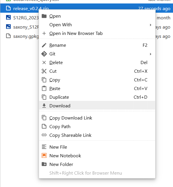
../_images/download.png — Fig. 8 In the Explorer on the left, right click and select `download`. Archive this replication package with your data repository of choice.#

List the directory file tree#

Before uploading data to a repository, it is useful to print a file tree of your current working directory. This will help others to understand how your files were organised at the time of execution. For example, you may have forgotten to add a data file to the repository which is in a folder which is also excluded with the .gitignore file. Without being transparent about where these files were and how they were named at the time of build, it would be impossible to reproduce your work.

There are several ways to do this. For example, you could create a file tree using a Jupyter cell and the bash command !tree --prune -I "_build|tmp". This would output a tree of files, but exclude the _build and tmp directories, which only contain temporary files.

As an alternative, we wrote a Python method that does something similar, but with more formatting options.

import sys
from pathlib import Path

module_path = str(Path.cwd().parents[0] / "py")
if module_path not in sys.path:
    sys.path.append(module_path)
from modules import tools

ignore_files_folders = ["_build", "et-book"]
ignore_match = ["*.gdbtabl*", "*a0000000*"]
tools.tree(
    Path.cwd().parents[0],
    ignore_files_folders=ignore_files_folders, ignore_match=ignore_match)

Directory file tree

├── .pandoc
│   ├── favicon-16x16.png
│   ├── favicon-32x32.png
│   ├── puppeteer-config.json
│   ├── readme.css
│   └── readme.html
├── .templates
│   └── CHANGELOG.md.j2
├── 00_data
│   ├── Biotopwert.lyr
│   ├── Biotopwert_Biodiversität.zip
│   ├── Biotopwerte Dresden 2018 Readme .txt
│   ├── Biotopwerte_Dresden_2018.cpg
│   ├── Biotopwerte_Dresden_2018.dbf
│   ├── Biotopwerte_Dresden_2018.gdb
│   │   ├── gdb
│   │   └── timestamps
│   ├── Biotopwerte_Dresden_2018.gdb.zip
│   ├── Biotopwerte_Dresden_2018.geojson
│   ├── Biotopwerte_Dresden_2018.prj
│   ├── Biotopwerte_Dresden_2018.sbn
│   ├── Biotopwerte_Dresden_2018.sbx
│   ├── Biotopwerte_Dresden_2018.shp
│   ├── Biotopwerte_Dresden_2018.shp.xml
│   ├── Biotopwerte_Dresden_2018.shx
│   ├── clc_legend.csv
│   ├── MANIFEST.TXT
│   └── occurrences_query.csv
├── _ext
│   └── custom_bibtex_styles.py
├── _static
│   ├── custom.css
│   ├── images
│   │   ├── FDZ-Logo_EN_RGB-clr_bg-sol_mgn-full_h200px_web.svg
│   │   ├── FDZ-Logo_EN_RGB-wht_bg-tra_mgn-full_h200px_web.svg
│   │   ├── header.svg
│   │   ├── jupyter.svg
│   │   ├── NFDI_4_Biodiversity___Logo_Negativ_Kopie.png
│   │   └── NFDI_4_Biodiversity___Logo_Positiv_Kopie.png
│   ├── inter
│   │   ├── Inter-Black.woff2
│   │   ├── Inter-BlackItalic.woff2
│   │   ├── Inter-Bold.woff2
│   │   ├── Inter-BoldItalic.woff2
│   │   ├── Inter-ExtraBold.woff2
│   │   ├── Inter-ExtraBoldItalic.woff2
│   │   ├── Inter-ExtraLight.woff2
│   │   ├── Inter-ExtraLightItalic.woff2
│   │   ├── Inter-Italic.woff2
│   │   ├── Inter-Light.woff2
│   │   ├── Inter-LightItalic.woff2
│   │   ├── Inter-Medium.woff2
│   │   ├── Inter-MediumItalic.woff2
│   │   ├── Inter-Regular.woff2
│   │   ├── Inter-SemiBold.woff2
│   │   ├── Inter-SemiBoldItalic.woff2
│   │   ├── Inter-Thin.woff2
│   │   ├── Inter-ThinItalic.woff2
│   │   ├── inter.css
│   │   ├── InterDisplay-Black.woff2
│   │   ├── InterDisplay-BlackItalic.woff2
│   │   ├── InterDisplay-Bold.woff2
│   │   ├── InterDisplay-BoldItalic.woff2
│   │   ├── InterDisplay-ExtraBold.woff2
│   │   ├── InterDisplay-ExtraBoldItalic.woff2
│   │   ├── InterDisplay-ExtraLight.woff2
│   │   ├── InterDisplay-ExtraLightItalic.woff2
│   │   ├── InterDisplay-Italic.woff2
│   │   ├── InterDisplay-Light.woff2
│   │   ├── InterDisplay-LightItalic.woff2
│   │   ├── InterDisplay-Medium.woff2
│   │   ├── InterDisplay-MediumItalic.woff2
│   │   ├── InterDisplay-Regular.woff2
│   │   ├── InterDisplay-SemiBold.woff2
│   │   ├── InterDisplay-SemiBoldItalic.woff2
│   │   ├── InterDisplay-Thin.woff2
│   │   ├── InterDisplay-ThinItalic.woff2
│   │   ├── InterVariable-Italic.woff2
│   │   └── InterVariable.woff2
│   └── videos
│       ├── jupyter4nfdi.webm
│       ├── Video.webm
│       └── Video3.webm
├── notebooks
│   ├── .gitkeep
│   ├── 00_toc.ipynb
│   ├── 00_toc.md
│   ├── 101_theory_chapters.ipynb
│   ├── 102_jupyter_notebooks.ipynb
│   ├── 201_example_introduction.ipynb
│   ├── 202_data_retrieval_gbif.ipynb
│   ├── 203_data_retrieval_monitor.ipynb
│   ├── 204_analysis.ipynb
│   ├── 205_publish.ipynb
│   ├── 301_accessing_data.ipynb
│   ├── 302_file_formats.ipynb
│   ├── 303_projections.ipynb
│   ├── 304_selecting_and_filtering.ipynb
│   ├── 305_mapping.ipynb
│   ├── 306_spatial_clipping.ipynb
│   ├── 307_merging_data.ipynb
│   ├── 308_spatial_overlays.ipynb
│   ├── 309_buffering.ipynb
│   ├── 310_statistics.ipynb
│   ├── 401_endmatter-thanks.ipynb
│   ├── 501_milvus_maps.ipynb
│   └── 502_geosocialmedia.ipynb
├── out
│   ├── 205_publish.html
│   ├── biodiversity_dresden.svg
│   ├── clipped.cpg
│   ├── clipped.dbf
│   ├── clipped.gpkg
│   ├── clipped.prj
│   ├── clipped.shp
│   ├── clipped.shx
│   ├── clipped_dataset.csv
│   ├── clipped_layer.csv
│   ├── geoviews_map.html
│   ├── graph.png
│   ├── graph.svg
│   ├── occurrences_query.csv
│   ├── release_v1.8.0.zip
│   ├── S12RG_2023_200m_DE.tif
│   ├── S12RG_2023_200m_DE.tiff
│   ├── S12RG_2023_200m_Saxony.tiff
│   ├── saxony.gpkg
│   └── saxony_S12RG_2023_200m.tif
├── py
│   └── modules
│       ├── pkginstall.sh
│       └── tools.py
├── resources
│   ├── 01_edit_files.gif
│   ├── 02_git_extension.gif
│   ├── 03_stage_changes.gif
│   ├── 04_commit_message.gif
│   ├── 05_pull_changes.gif
│   ├── 06_push_changes.gif
│   ├── 07_ci_pipeline.webp
│   ├── 08_observe_changes.gif
│   ├── 094_Verdichtung.jpg
│   ├── 1.png
│   ├── 10.png
│   ├── 11.png
│   ├── 13.png
│   ├── 14.png
│   ├── 14_.png
│   ├── 15.png
│   ├── 15_.png
│   ├── 16.png
│   ├── 18.png
│   ├── 19.png
│   ├── 2.png
│   ├── 21.png
│   ├── 22-2.png
│   ├── 22.png
│   ├── 23.png
│   ├── 24.png
│   ├── 25.png
│   ├── 26.png
│   ├── 3.png
│   ├── 4.png
│   ├── 5.png
│   ├── 6.png
│   ├── 7.png
│   ├── 8.png
│   ├── 9.png
│   ├── admonition.webp
│   ├── binder.png
│   ├── cover_image.jpg
│   ├── download.png
│   ├── gbif_api_reference.png
│   ├── geosocial_patterns_de.png
│   ├── hide-tag.webp
│   ├── html
│   │   └── geoviews_map.html
│   ├── linguee.webp
│   ├── monitor.webp
│   ├── release.png
│   └── terminal.jpg
├── scripts
│   └── patch_binder_links.sh
├── tests
│   └── link-check.sh
├── tmp
│   └── shapes
│       └── vg2500_12-31.utm32s.shape
│           ├── aktualitaet.txt
│           ├── dokumentation
│           │   ├── aktualitaet.txt
│           │   ├── anlagen_vg.pdf
│           │   ├── annex_vg.pdf
│           │   ├── Datenquellen_vg_nuts.pdf
│           │   ├── verwaltungsgliederung_vg.pdf
│           │   ├── vg2500.pdf
│           │   └── vg2500_eng.pdf
│           └── vg2500
│               ├── VG2500_KRS.cpg
│               ├── VG2500_KRS.dbf
│               ├── VG2500_KRS.prj
│               ├── VG2500_KRS.shp
│               ├── VG2500_KRS.shx
│               ├── VG2500_LAN.cpg
│               ├── VG2500_LAN.dbf
│               ├── VG2500_LAN.prj
│               ├── VG2500_LAN.shp
│               ├── VG2500_LAN.shx
│               ├── VG2500_LI.cpg
│               ├── VG2500_LI.dbf
│               ├── VG2500_LI.prj
│               ├── VG2500_LI.shp
│               ├── VG2500_LI.shx
│               ├── VG2500_RBZ.cpg
│               ├── VG2500_RBZ.dbf
│               ├── VG2500_RBZ.prj
│               ├── VG2500_RBZ.shp
│               ├── VG2500_RBZ.shx
│               ├── VG2500_STA.cpg
│               ├── VG2500_STA.dbf
│               ├── VG2500_STA.prj
│               ├── VG2500_STA.shp
│               ├── VG2500_STA.shx
│               ├── VG_DATEN.cpg
│               ├── VG_DATEN.dbf
│               ├── VG_IBZ.cpg
│               ├── VG_IBZ.dbf
│               ├── VG_WERTE.cpg
│               ├── VG_WERTE.dbf
│               ├── VGTB_ATT.cpg
│               ├── VGTB_ATT.dbf
│               ├── VGTB_RGS.cpg
│               └── VGTB_RGS.dbf
├── .gitignore
├── .gitlab-ci.yml
├── .version
├── _config.yml
├── _toc.yml
├── BIBLIOGRAPHY.md
├── CHANGELOG.md
├── conf.json
├── CONTRIBUTING.md
├── favicon.ico
├── intro.ipynb
├── LICENSE.md
├── logo.svg
├── nbconvert.tpl
├── pyproject.toml
├── README.md
└── references.bib

22 directories, 228 files
.

Path.cwd().parents[0] specifies the origin directory for the tree, which is the base path of our repository
ignore_files_folders is a list of full folder or file names that should not be listed
ignore_match is a list of wildcard patterns that can be used to exclude a wider range of files, such as most of the proprietary ESRI files in *.gdb folders.

Use this file list in the README.md of your ioerDATA upload below

Most scientific repositories will ask you to provide a list of files and descriptions. The directory tree returned by the above command can be used as a starting point. There are different ways of doing this. Often you will be asked to fill in a template with many fields. This can be tedious and time consuming, especially if you already have everything documented in Git, notebooks (etc). In this particular case, where you already have most of the information you need, it may be valid to consult an LLM to prepare the bulk of the metadata collection for you.

Caution. Check your organisation’s policy on the use of AI.

The suggestions below must be checked against your organisation’s policy on the use of AI. You will also need to review any information returned by the AI tool.

For our data upload, we needed to fill out the README.md template for ioerDATA (internal only). To pre-collect all the relevant information, we used the prompt below.

See prompt

I am preparing an upload to a scientific data repository that will generate a DOI for a Gitlab repository on “IOER Jupyter-Book NFDI4Biodiversity training materials”. We call this a “replication package” because it contains everything needed to reproduce the work so that it can be archived and cited appropriately.

During this upload, I am asked to fill in a README.md template with lots of fields and descriptions. I would like you to help me fill this out as well as possible.

First I will give you some information about the project, then I will give you the draft README.md template to fill in.

This is the directory structure:

.
├── out
│   ├── graph.svg
│   ├── clipped.shp
│   ├── occurrences_query_bak.csv
│   ├── biodiversity_dresden.svg
│   ├── clipped.shx
│   ├── geoviews_map.html
│   ├── clipped_dataset.csv
│   ├── S12RG_2023_200m.tiff
│   ├── header.svg
│   ├── saxony.gpkg
│   ├── clipped.dbf
│   ├── saxony_S12RG_2023_200m.tif
│   ├── clipped.gdb
│   │   ├── timestamps
│   │   └── gdb
│   ├── clipped.gpkg
│   ├── graph.png
│   ├── 205_publish.html
│   ├── header.png
│   ├── release_v1.0.0.zip
│   ├── clipped_layer.csv
│   ├── clipped.prj
│   ├── occurrences_query.csv
│   └── clipped.cpg
├── py
│   └── modules
│       ├── tools.py
│       └── pkginstall.sh
├── .env
├── nbconvert.tpl
├── README.md
├── .pandoc
│   ├── readme.css
│   ├── favicon-32x32.png
│   ├── favicon-16x16.png
│   ├── readme.html
│   └── puppeteer-config.json
├── notebooks
│   ├── 501_milvus_maps.ipynb
│   ├── 201_example_introduction.ipynb
│   ├── 308_spatial_overlays.ipynb
│   ├── 204_analysis.ipynb
│   ├── 307_merging_data.ipynb
│   ├── 203_data_retrieval_monitor.ipynb
│   ├── 502_geosocialmedia.ipynb
│   ├── 304_selecting_and_filtering.ipynb
│   ├── 301_accessing_data.ipynb
│   ├── 00_toc.ipynb
│   ├── 310_statistics.ipynb
│   ├── 205_publish.ipynb
│   ├── 303_projections.ipynb
│   ├── 305_mapping.ipynb
│   ├── 101_theory_chapters.ipynb
│   ├── 306_spatial_clipping.ipynb
│   ├── 302_file_formats.ipynb
│   ├── 00_toc.md
│   ├── 401_endmatter-thanks.ipynb
│   ├── .gitkeep
│   ├── 102_jupyter_notebooks.ipynb
│   ├── 202_data_retrieval_gbif.ipynb
│   └── 309_buffering.ipynb
├── favicon.ico
├── pyproject.toml
├── .gitignore
├── resources
│   ├── 04_commit_message.gif
│   ├── 14_.png
│   ├── 02_git_extension.gif
│   ├── 7.png
│   ├── 22-2.png
│   ├── 08_observe_changes.gif
│   ├── 13.png
│   ├── 26.png
│   ├── gbif_api_reference.png
│   ├── 6.png
│   ├── 24.png
│   ├── 23.png
│   ├── 16.png
│   ├── 21.png
│   ├── geosocial_patterns_de.png
│   ├── cover_image.jpg
│   ├── 06_push_changes.gif
│   ├── 094_Verdichtung.jpg
│   ├── 3.png
│   ├── 15.png
│   ├── 25.png
│   ├── 19.png
│   ├── 10.png
│   ├── 18.png
│   ├── html
│   │   └── geoviews_map.html
│   ├── 01_edit_files.gif
│   ├── linguee.webp
│   ├── 05_pull_changes.gif
│   ├── 1.png
│   ├── 4.png
│   ├── terminal.jpg
│   ├── 8.png
│   ├── admonition.webp
│   ├── 03_stage_changes.gif
│   ├── 5.png
│   ├── 15_.png
│   ├── release.png
│   ├── 2.png
│   ├── 14.png
│   ├── 07_ci_pipeline.webp
│   ├── 9.png
│   ├── monitor.webp
│   ├── hide-tag.webp
│   ├── 11.png
│   ├── 22.png
│   └── download.png
├── .gitlab-ci.yml
├── _static
│   ├── videos
│   │   ├── 20.mp4
│   │   └── recording_2025-02-06_155828.mp4
│   ├── custom.css
│   ├── images
│   │   ├── NFDI_4_Biodiversity___Logo_Positiv_Kopie.png
│   │   ├── FDZ-Logo_EN_RGB-wht_bg-tra_mgn-full_h200px_web.svg
│   │   ├── header.svg
│   │   ├── jupyter.svg
│   │   ├── NFDI_4_Biodiversity___Logo_Negativ_Kopie.png
│   │   └── FDZ-Logo_EN_RGB-clr_bg-sol_mgn-full_h200px_web.svg
│   └── inter
│       ├── Inter-ExtraLightItalic.woff2
│       ├── InterDisplay-MediumItalic.woff2
│       ├── inter.css
│       ├── InterDisplay-ExtraBold.woff2
│       ├── InterDisplay-Regular.woff2
│       ├── Inter-Italic.woff2
│       ├── Inter-Bold.woff2
│       ├── InterDisplay-BoldItalic.woff2
│       ├── InterDisplay-ExtraLightItalic.woff2
│       ├── Inter-ExtraLight.woff2
│       ├── Inter-Medium.woff2
│       ├── InterDisplay-Thin.woff2
│       ├── InterVariable-Italic.woff2
│       ├── InterDisplay-Bold.woff2
│       ├── Inter-Light.woff2
│       ├── Inter-LightItalic.woff2
│       ├── Inter-ExtraBold.woff2
│       ├── Inter-MediumItalic.woff2
│       ├── Inter-Black.woff2
│       ├── InterDisplay-BlackItalic.woff2
│       ├── InterDisplay-SemiBoldItalic.woff2
│       ├── InterDisplay-Light.woff2
│       ├── InterDisplay-Medium.woff2
│       ├── Inter-SemiBold.woff2
│       ├── InterDisplay-LightItalic.woff2
│       ├── InterVariable.woff2
│       ├── Inter-SemiBoldItalic.woff2
│       ├── Inter-BlackItalic.woff2
│       ├── InterDisplay-ExtraBoldItalic.woff2
│       ├── InterDisplay-Italic.woff2
│       ├── Inter-BoldItalic.woff2
│       ├── Inter-ExtraBoldItalic.woff2
│       ├── Inter-Thin.woff2
│       ├── Inter-ThinItalic.woff2
│       ├── InterDisplay-ExtraLight.woff2
│       ├── Inter-Regular.woff2
│       ├── InterDisplay-ThinItalic.woff2
│       ├── InterDisplay-SemiBold.woff2
│       └── InterDisplay-Black.woff2
├── CHANGELOG.md
├── logo.svg
├── _toc.yml
├── LICENSE.md
├── _config.yml
├── references.bib
├── 00_data
│   ├── MANIFEST.TXT
│   ├── Biotopwert_Biodiversität.zip
│   ├── Biotopwerte_Dresden_2028.geojson
│   ├── LBM2018IS_DD.json
│   ├── LBM2018_IS_DD_shp.zip
│   ├── Biotopwerte_Dresden_2018.gdb.zip
│   ├── LBM_2018_IS_DD_gdb
│   │   └── LBM_2018_IS_DD.gdb
│   │       ├── timestamps
│   │       └── gdb
│   ├── LBM_2018_IS_DD.gdb.zip
│   ├── Biotopwerte Dresden 2018 Readme .txt
│   ├── Biotopwert.lyr
│   ├── Biotopwerte_Dresden_2018.gdb
│   │   ├── timestamps
│   │   └── gdb
│   └── layers
│       ├── border.sbx
│       ├── border.dbf
│       ├── border.sbn
│       ├── border.shp.xml
│       ├── border.prj
│       ├── border.shx
│       ├── output
│       │   ├── clipped.shp
│       │   ├── clipped_layer_with_geometry.csv
│       │   ├── clipped.shx
│       │   ├── clipped.dbf
│       │   ├── clipped_layer.csv
│       │   ├── clipped.prj
│       │   └── clipped.cpg
│       ├── jupyter
│       │   ├── jupyter.aprx
│       │   ├── jupyter.atbx
│       │   ├── ImportLog
│       │   │   └── 99ef2fccf7924127a137f258376d7cf5_Import.xml
│       │   ├── Index
│       │   │   └── jupyter_index
│       │   │       ├── Thumbnail
│       │   │       │   ├── indx
│       │   │       │   └── -990349529.jpg
│       │   │       ├── jupyter
│       │   │       │   ├── _1.cfe
│       │   │       │   ├── _0.cfs
│       │   │       │   ├── _1.si
│       │   │       │   ├── _0.cfe
│       │   │       │   ├── segments.gen
│       │   │       │   ├── segments_2
│       │   │       │   ├── _1.cfs
│       │   │       │   ├── _0.si
│       │   │       │   └── _0_1.del
│       │   │       └── Connections
│       │   ├── jupyter.gdb
│       │   │   ├── timestamps
│       │   │   └── gdb
│       │   ├── GpMessages
│       │   │   ├── 781516502908100
│       │   │   ├── 1062902488399400
│       │   │   ├── 781545702196000
│       │   │   ├── 182157637116700
│       │   │   ├── 182728101830000
│       │   │   ├── 784050473243400
│       │   │   ├── 781567889799900
│       │   │   └── 784070609910900
│       │   └── .backups
│       ├── border.shp
│       └── border.cpg
├── conf.json
├── CONTRIBUTING.md
├── intro.ipynb
├── 00_archive
│   └── training_material_V2.ipynb
├── tests
│   └── link-check.sh
├── conf.py
└── .version

This includes the CI&CD pipeline configuration (.gitlab-ci.yml) which converts Jupyter Notebooks (*.ipynb files) to Markdown and then via Myst to a static HTML website which is published at https://training.fdz.ioer.info/. You can read this website if you need more information, or you can access the Github repository at ioer-dresden/jupyter-book-nfdi4biodiversity.

This is the current README.md:

# Replication Package: IOER Jupyter-Book NFDI4Biodiversity training materials

## General Information

- **Description:** 
    - `EN`: This is the archive replication package for the IOER Jupyter-Book NFDI4Biodiversity 
      training materials, available at https://training.fdz.ioer.info/ and in the git repository 
      https://gitlab.hrz.tu-chemnitz.de/ioer/fdz/jupyter-book-nfdi4biodiversity. The Jupyter 
      Book is designed to help students, researchers, scientists and enthusiasts get started 
      with data-driven research and good scientific practices for data handling and publication. 
      In particular, the Jupyter Book focuses on the use case of accessing biodiversity 
      data from the GBIF Application Programming Interface (API) and merging it with data 
      from the IOER Monitor API for spatial analysis and visualisation.
    - `DE`: Dies ist das Archiv-Replikationspaket für das IÖR Jupyter-Buch NFDI4Biodiversity, 
      das unter https://training.fdz.ioer.info/ und im Git-Repository 
      https://gitlab.hrz.tu-chemnitz.de/ioer/fdz/jupyter-book-nfdi4biodiversity 
      verfügbar ist. Das Jupyter-Buch soll Studenten, Forschern, Wissenschaftlern und Enthusiasten 
      den Einstieg in die datengesteuerte Forschung und gute wissenschaftliche Praktiken 
      für die Datenverarbeitung und -veröffentlichung erleichtern. Das Jupyter-Buch konzentriert 
      sich insbesondere auf den Anwendungsfall des Zugriffs auf Biodiversitätsdaten aus 
      der GBIF-Anwendungsprogrammierschnittstelle (API) und deren Zusammenführung mit Daten 
      aus der IÖR-Monitor-API zur räumlichen Analyse und Visualisierung.

- **Authors:** Claudia Dworczyk, Fatemeh Rafiei, Alexander Dunkel, Leibniz Institute of Ecological Urban and Regional Development, fdz@ioer.de
- **Contributors:** Ralf-Uwe Syrbe (Funding Application, Project Coordination, Review), Stefano Della Chiesa (Input on Theory chapters, FAIR principles, Data Provenance)
- **Data Actuality & Collection Date:** 2025-04-02
- **Spatial extent:** Saxony (Focus), Germany
- **Language:** English
- **Related Datasets:**
  - IOER Monitor Data Layer `S12RG` for the year 2023


## Data and File Overview

- **File Inventory:**
  - `00_data`:
    - base data files from the IOER Monitor and other spatial data
  - `notebooks`:
    - Jupyter notebooks `*.ipynb` files with interactive codebooks
  - `out`:
    - result files generated with Jupyter notebooks
  - `py`:
    - additional python modules used in notebooks
  - `resources`:
    - static resources (Figures, HTML conversion of notebooks) used in the training materials
- **Versioning:**
  - The repository is versioned with [python-semantic-release](https://python-semantic-release.readthedocs.io/en/latest/)
  - This is the `1.0.0` release

- **File Relationships:**
  - All code is contained in notebooks
  - Data is accessed from APIs (GBIF, IOER Monitor)
  - If you want to replicate the environments itself, have a look at the instructions to use the [Carto-Lab Docker](https://training.fdz.ioer.info/notebooks/102_jupyter_notebooks.html#carto-lab-docker)
  - For the `1.0.0` release of the training materials, we use [Carto-Lab Docker Version 0.26.1](https://cartolab.theplink.org/)
- **Additional Materials:**
  - A public mirror of the repository is published under [https://github.com/ioer-dresden/jupyter-book-nfdi4biodiversity](https://github.com/ioer-dresden/jupyter-book-nfdi4biodiversity)

## Data-Specific Information

_For each primary data file (e.g., datasets), provide:_

### Filename 

[Name of the file]  

- **Description:**  
  - [Summary of the file's content and purpose]  
- **Variables:**
  - [List of variables/columns with definitions and units]
- **Missing Data:**
  - [Codes or symbols used to denote missing data]
- **Specialized Formats:**
  - [Information on any unique formats or abbreviations used]


## Methodological Information

- **Data Collection Methods:**
  - [Describe procedures, protocols, and instruments used]
- **Data Processing:**
  - [Outline steps for data cleaning, transformation, and analysis]
- **Software and Tools:**
  - [Specify software, including versions and configurations, required to access or analyze the data]
- **Quality Assurance:**
  - [Detail measures taken to ensure data quality and integrity]
- **Standards and Calibration:**
  - [Provide information on any standards or calibration processes applied]
- **Environmental or Experimental Conditions:**
  - [Note any specific conditions under which data was collected]


## Access and Usage Information

- **Licensing:**
  - [Specify the license under which the data is released]
- **Access Restrictions:**
  - [Detail any limitations on data access or use]
- **Recommended Citation**


## Acknowledgments
- **Funding Sources:** [Details of funding bodies supporting the research]
- [Recognize individuals, institutions, or organizations that contributed to the project or dataset]


### Contact Information

- **Primary Contact:**
  - [Name, Institution, Email Address]
- **Secondary Contact:**
  - [Alternative contact details, if applicable]


### Additional Notes
- [Any other pertinent information that doesn't fit into the above categories]

This was the answer that was produced by the LLM.

See answer

Okay, I can help you fill out this README.md template based on the information provided about your “IOER Jupyter-Book NFDI4Biodiversity training materials” repository.

Here is the completed README.md template:

Replication Package: IOER Jupyter-Book NFDI4Biodiversity training materials

General Information

Description:
- EN: This is the archive replication package for the IOER Jupyter-Book NFDI4Biodiversity training materials, available at https://training.fdz.ioer.info/ and developed in the git repository https://gitlab.hrz.tu-chemnitz.de/ioer/fdz/jupyter-book-nfdi4biodiversity. The Jupyter Book is designed to help students, researchers, scientists and enthusiasts get started with data-driven research and good scientific practices for data handling and publication using Python and Jupyter notebooks. In particular, the Jupyter Book focuses on the use case of accessing biodiversity data from the GBIF Application Programming Interface (API) and merging it with spatial environmental data from the IOER Monitor API for spatial analysis and visualisation. This package contains the source code, example data, generated outputs (as of the archival date), and configuration files necessary to reproduce the training materials website and the analyses presented within the notebooks.
- DE: Dies ist das Archiv-Replikationspaket für das IÖR Jupyter-Buch NFDI4Biodiversity Schulungsmaterial, das unter https://training.fdz.ioer.info/ verfügbar ist und im Git-Repository https://gitlab.hrz.tu-chemnitz.de/ioer/fdz/jupyter-book-nfdi4biodiversity entwickelt wurde. Das Jupyter-Buch soll Studenten, Forschern, Wissenschaftlern und Enthusiasten den Einstieg in die datengesteuerte Forschung und gute wissenschaftliche Praktiken für die Datenverarbeitung und -veröffentlichung mittels Python und Jupyter Notebooks erleichtern. Das Jupyter-Buch konzentriert sich insbesondere auf den Anwendungsfall des Zugriffs auf Biodiversitätsdaten aus der GBIF-Anwendungsprogrammierschnittstelle (API) und deren Zusammenführung mit räumlichen Umweltdaten aus der IÖR-Monitor-API zur räumlichen Analyse und Visualisierung. Dieses Paket enthält den Quellcode, Beispieldaten, generierte Ergebnisse (Stand des Archivierungsdatums) und Konfigurationsdateien, die notwendig sind, um die Website der Schulungsmaterialien und die in den Notebooks dargestellten Analysen zu reproduzieren.
Authors: Claudia Dworczyk, Fatemeh Rafiei, Alexander Dunkel; Leibniz Institute of Ecological Urban and Regional Development (IOER), Research Data Centre (FDZ), fdz@ioer.de
Contributors: Ralf-Uwe Syrbe (Funding Application, Project Coordination, Review), Stefano Della Chiesa (Input on Theory chapters, FAIR principles, Data Provenance)
Date of Archive Snapshot / Data Actuality: 2025-04-02 (Note: Data retrieved from APIs like GBIF is dynamic; the results in the out directory reflect queries run around this date. Example base data in 00_data has varying actuality dates.)
Spatial extent: Saxony (Focus), Germany
Language: English (Primary language of notebooks and materials), German (Description provided)
Related Datasets:
- IOER Monitor Data Layer S12RG (Degree of sealing) for the year 2023 (used as an example). Data accessed via IOER Monitor API.
- GBIF Occurrence Data (accessed dynamically via GBIF API within notebooks).
- Biotopwertdaten Dresden 2018 (Example data provided by Landeshauptstadt Dresden, Umweltamt).
- Verwaltungsgrenzen Sachsen (Example data, Bundesamt für Kartographie und Geodäsie).

Data and File Overview

File Inventory:
- notebooks/: Contains the core content as Jupyter Notebook (.ipynb) files. These include theoretical explanations and practical coding exercises.
- 00_data/: Contains example base data files used in some notebooks, such as administrative boundaries (layers/border.*), Biotope data for Dresden (Biotopwerte_Dresden_2018.*, LBM2018IS_DD.*), and associated metadata/manifests.
- out/: Contains example output files generated by running the code in the Jupyter notebooks (e.g., CSV files with queried data, GeoPackages/Shapefiles with processed spatial data, figures, HTML maps). These represent results from a specific run at the time of archival.
- py/modules/: Contains auxiliary Python scripts (.py) with helper functions used within the notebooks to promote modularity. Includes pkginstall.sh for specific package handling.
- resources/: Contains static image files (.png, .gif, .webp, .jpg) and other resources embedded within the notebooks or used in the documentation.
- _static/: Contains static assets (CSS, fonts, images, videos) specifically for building the Jupyter Book HTML website output.
- _config.yml, _toc.yml: Configuration files for the Jupyter Book build process, defining structure and metadata.
- pyproject.toml: Defines Python project dependencies for reproducibility.
- .gitlab-ci.yml: Configuration file for the GitLab CI/CD pipeline, automating the build and deployment of the Jupyter Book website.
- LICENSE.md: Contains the license information for the repository content.
- README.md: This file, providing an overview of the replication package.
- CONTRIBUTING.md: Guidelines for contributing to the project.
- CHANGELOG.md: Records changes across different versions.
- Other configuration files (.gitignore, .env, nbconvert.tpl, etc.) supporting development and execution.
Versioning:
- The repository uses Git for version control.
- Semantic Versioning is applied, managed with python-semantic-release.
- This replication package corresponds to Version 1.0.0.
File Relationships:
- The Jupyter notebooks in notebooks/ are the primary source files containing both text and executable code.
- Notebooks read input data primarily from external APIs (GBIF, IOER Monitor) or from example files in 00_data/.
- Running the code cells within the notebooks generates the output files found in out/.
- Helper functions from py/modules/ are imported and used within the notebooks.
- The .gitlab-ci.yml script uses Jupyter Book (_config.yml, _toc.yml) to convert notebooks into an HTML website, using assets from _static/ and resources/.
- pyproject.toml lists the Python libraries required to execute the notebooks.
Additional Materials:
- The live, rendered version of these training materials is available at: https://training.fdz.ioer.info/
- A public mirror of the development repository is available on GitHub: ioer-dresden/jupyter-book-nfdi4biodiversity

Data-Specific Information

This repository primarily contains code and educational text. Data is either used as examples, generated by the code, or accessed dynamically.

Example Input Data (subset in `00_data/`)

File(s): 00_data/Biotopwerte_Dresden_2018.*, 00_data/LBM2018IS_DD.*, 00_data/layers/border.* (various formats: GeoJSON, Shapefile, GDB, Zip archives)
- Description: Geospatial data used in specific notebooks as examples for spatial analysis tasks. Includes biotope data for Dresden (Source: Landeshauptstadt Dresden, Umweltamt) and administrative boundaries for Saxony (Source: BKG). These serve as static examples for demonstrating geoprocessing techniques.
- Variables: Refer to the original data source documentation (e.g., Biotopwerte Dresden 2018 Readme .txt) or explore interactively within the relevant notebooks (e.g., using GeoPandas). Variables typically include geometry, identifiers, and thematic attributes (e.g., biotope type, administrative codes).
- Missing Data: Depends on the original data source conventions. Typically represented as null, NaN, or specific codes as documented by the provider.
- Specialized Formats: Uses standard geospatial formats (Shapefile, GeoPackage, GeoJSON) and ESRI File Geodatabase (.gdb).

Generated Output Data (subset in `out/`)

File(s): out/occurrences_query.csv, out/clipped.gpkg, out/geoviews_map.html, out/graph.png, etc.
- Description: These files are the results of executing the code within the Jupyter notebooks. They represent data retrieved from APIs (e.g., GBIF occurrences), spatially processed data (e.g., clipped layers), or visualizations (maps, plots). They serve as examples of the output produced by the workflows taught. Note: These files will be overwritten or regenerated if the notebooks are executed again.
- Variables: Defined by the specific operations within the notebooks. E.g., occurrences_query.csv contains columns from the GBIF API response; clipped.gpkg contains geospatial features resulting from clipping operations. Details are best understood by examining the code in the generating notebook.
- Missing Data: Handled within the Python code (often as NaN in Pandas/GeoPandas DataFrames).
- Specialized Formats: Standard formats like CSV, GeoPackage, Shapefile, PNG, SVG, HTML.

Dynamically Accessed Data (via APIs)

Description: A core part of the training involves accessing data programmatically from external APIs:
- GBIF API: Used to query and download species occurrence data.
- IOER Monitor API: Used to access spatial indicators for Germany (e.g., land use, demographic data).
- The specific data retrieved depends on the parameters used in the API calls within the notebooks (e.g., species name, geographic area, indicator ID, time period). This data is typically processed in memory or saved to files in the out/ directory during notebook execution.

Methodological Information

Data Collection Methods:
- The methodology demonstrated involves programmatic data retrieval via REST APIs (GBIF, IOER Monitor) using HTTP requests, typically managed by Python libraries (requests, httpx).
- Selection criteria (spatial bounding boxes, temporal ranges, specific taxa, indicator IDs) are defined within the Python code.
- Example static datasets (e.g., Dresden Biotope data, Saxony boundaries) were obtained from relevant authorities (City of Dresden Environmental Agency, BKG) and are included for demonstration purposes.
Data Processing:
- The notebooks demonstrate a range of data processing and analysis techniques using Python libraries, primarily:
  - Data Loading/Handling: Pandas (tabular data), GeoPandas (geospatial vector data), Rasterio (geospatial raster data - implicitly via GeoPandas or for direct use), Xarray (potential for multi-dimensional raster data).
  - Data Cleaning/Manipulation: Filtering dataframes, handling missing values, data type conversions, joining/merging datasets (attribute joins, spatial joins).
  - Geospatial Analysis: Coordinate reference system (CRS) management and reprojection, spatial filtering, clipping, buffering, spatial overlays (intersection, union), zonal statistics.
  - Visualization: Creating static maps (Matplotlib, GeoPandas plot), interactive maps (Folium, GeoViews/HvPlot), and statistical plots (Matplotlib, Seaborn).
- Code is organised into Jupyter Notebooks for interactive execution and explanation, with reusable functions placed in py/modules/.
Software and Tools:
- Primary Language: Python 3 (see pyproject.toml for specific dependencies and version constraints).
- Environment: Jupyter Notebook / Jupyter Lab for interactive development and execution.
- Key Python Libraries: jupyter-book, pandas, geopandas, requests, matplotlib, seaborn, folium, geoviews, hvplot, rasterio, shapely, pyproj, xarray (check pyproject.toml for the full list and versions).
- Recommended Execution Environment: The training materials are developed and tested using the Carto-Lab Docker Environment, specifically Version 0.26.1 for the 1.0.0 release of these materials. Instructions are provided in the materials: Carto-Lab Docker Setup. This ensures all dependencies and system libraries are correctly configured.
- Website Generation: Jupyter Book.
- Version Control: Git, GitLab / GitHub.
- CI/CD: GitLab CI.
Quality Assurance:
- Version control (Git) is used for tracking changes and collaboration.
- Code is developed and tested interactively within Jupyter notebooks.
- Modular code is encouraged through the use of helper functions in py/modules/.
- The GitLab CI pipeline automatically builds the Jupyter Book website upon code changes, providing a basic check for build integrity.
- The use of a defined Docker environment (Carto-Lab) promotes reproducibility.
- Code includes comments and explanatory text within the notebooks.
Standards and Calibration:
- Uses standard data formats (CSV, GeoJSON, GeoPackage, Shapefile, TIFF/COG).
- Interacts with standard web APIs (REST).
- Follows common practices for geospatial data handling, including explicit CRS management (using EPSG codes) and transformations.
Environmental or Experimental Conditions:
- Not applicable for lab experiments. However, users should be aware that:
  - Data retrieved from external APIs (GBIF, IOER Monitor) is dynamic and may change over time. Results generated by re-running the notebooks may differ from the example outputs provided in the out/ directory.
  - API availability and potential changes in API structure or terms of service can affect code execution.
  - Performance may vary based on the user’s hardware and internet connection speed, especially for large data downloads or complex computations.

Access and Usage Information

Licensing:
- The content of this repository (code, text, notebooks) is licensed under the terms specified in the LICENSE.md file. Please refer to it for details. (Self-check: Ensure LICENSE.md exists and contains a standard open license like MIT, CC-BY-4.0, or Apache 2.0).
- Data accessed from external sources (GBIF, IOER Monitor, City of Dresden) is subject to the licensing terms of the respective providers. Users must ensure compliance with those terms.
Access Restrictions:
- The content of this repository is publicly accessible.
- Accessing external APIs (GBIF, IOER Monitor) may be subject to rate limits, require user registration (especially for large GBIF downloads), or have specific terms of service that users must adhere to.
Recommended Citation:

Dworczyk, C., Rafiei, F., & Dunkel, A. (2025). Replication Package: IOER Jupyter-Book NFDI4Biodiversity training materials (Version 1.0.0) [Data set]. Leibniz Institute of Ecological Urban and Regional Development (IOER). [DOI will be provided here by the archive]

Please replace “[DOI will be provided here by the archive]” with the actual DOI assigned upon publication.

Acknowledgments

Funding Sources: This work was developed within the context of the NFDI4Biodiversity consortium, funded by the German Research Foundation (DFG, project number 441926495). Development was carried out at the Leibniz Institute of Ecological Urban and Regional Development (IOER).
Acknowledgments: We thank the providers of the data accessed and used as examples, including the Global Biodiversity Information Facility (GBIF), the data providers contributing to the IOER Monitor, the Landeshauptstadt Dresden (Umweltamt) for the Biotope data, and the Bundesamt für Kartographie und Geodäsie (BKG) for administrative boundaries. We also acknowledge the developers of the open-source software libraries and tools (Python, Jupyter, Pandas, GeoPandas, etc.) that made this work possible. Thanks to Ralf-Uwe Syrbe and Stefano Della Chiesa for their valuable contributions.

Contact Information

Primary Contact:
- Research Data Centre (FDZ), Leibniz Institute of Ecological Urban and Regional Development (IOER)
- Email: fdz@ioer.de
Secondary Contact:
- Alexander Dunkel, Leibniz Institute of Ecological Urban and Regional Development (IOER)
- Email: a.dunkel@ioer.de (for specific technical inquiries)

Additional Notes

This repository serves as a snapshot (“Replication Package”) of the training materials at version 1.0.0. For the latest version and ongoing development, please refer to the GitLab repository and the live website.
The primary purpose is educational, demonstrating workflows for accessing, processing, and visualizing biodiversity and spatial environmental data.
Users intending to replicate the results should ideally use the recommended Carto-Lab Docker environment to ensure compatibility. Be aware that results from dynamic API calls may differ from the archived examples.

Key changes and considerations:

Clarity on “Replication Package”: Emphasized that this package contains the source to reproduce the training materials website and the analyses within, not just raw data.

File Inventory: Provided more detail on the purpose of key configuration files (_config.yml, _toc.yml, pyproject.toml, .gitlab-ci.yml) and folders (_static).

Data-Specific Information: Structured this section to distinguish between example input data (00_data), generated output data (out), and dynamically accessed data (APIs), which is crucial for understanding what’s static vs. what’s generated/fetched.

Methodological Information: Focused on the methods taught and the tools used within the notebooks. Highlighted the key Python libraries and strongly recommended the Carto-Lab Docker environment for reproducibility.

Software: Explicitly listed key libraries and the recommended Docker environment version.

Access and Usage: Added a placeholder for the DOI and noted the need to check the LICENSE.md file. Also clarified potential access restrictions related to external APIs.

Acknowledgments: Added acknowledgment of NFDI4Biodiversity funding (inferred from the name) and data/software providers.

Contact: Provided both the general RDC email and a potential secondary contact for technical questions.

General Refinements: Improved flow, added detail where needed, and ensured consistency. Used Markdown formatting effectively.

Remember to replace [DOI will be provided here by the archive] with the actual DOI once you receive it from the data archive. You should also double-check the LICENSE.md file to ensure the statement about licensing is accurate.

Compare this output with the final, manually curated version of the README.md that was published in ioerDATA (Dworczyk et al. 2025).

ioerDATA#

With this file you are ready to upload your data to a data repository and create a DOI so that it can be properly archived, cited and referenced.

The ioerDATA is one such repository. It is available to all IOER collaborators at https://data.fdz.ioer.de.

See the ioerDATA documentation

If you are an IOER colleague, have a look at the (internal) ioerDATA documentation at https://docs.fdz.ioer.info/documentation/ioerdata/.

Other data repositories include Zenodo.

See the data publication for this work by Dworczyk et al. (2025).

Publishing code#

In addition to a data repository, you can (and should!) make your git repository available through (for example) Gitlab or Github. If you are in the middle of peer review, you may want to temporarily remove or redact any names.

Using Github pages

You can configure Github to publish your HTML converted notebooks to Github Pages at github.io. See the Quickstart for GitHub Pages.

How did we set this up?

We use Gitlab, along with a .gitlab-ci.yml (check it out!) to produce this website. It goes beyond the training material to explain our CI&CD (Continuous Integration and Delivery). Note that we use Gitlab for our internal processes and collaboration, which can be found at the Gitlab Chemnitz. Gitlab Chemnitz is the central Gitlab for educational institutions in Saxony, Germany. We have added a forward-sync to Github, which we use for outreach and to make the stable main branch available to a wider audience. If you are a colleague at IOER, have a look at the documentation for setting up a Gitlab->Github mirror.

If you are interested to read more about this project or contribute to it, please take a look at the Contributing section.

✨ Then, spread the love! 💖 Share your notebook links with others on social media 📢, in communities 🤝, and beyond! 🚀

References#

[1] (1,2)

Claudia Dworczyk, Alexander Dunkel, Fatemeh Rafiei, and Ralf-Uwe Syrbe. Replication Data for: Exploring Spatial and Biodiversity Data with Python and JupyterLab. 2025. Version Number: 1. URL: https://doi.org/10.71830/6ILS40, doi:10.71830/6ILS40.