Selecting and Filtering Data#
Summary
When working with large datasets, processing and visualizing all the data in Jupyter can be time-consuming or may fail entirely. To overcome this, it’s practical to limit the data by selecting only the portions relevant to the analysis.
Load the data
import geopandas as gp
import pandas as pd
from pathlib import Path
INPUT = Path.cwd().parents[0] / "00_data"
gdb_path = INPUT / "Biotopwerte_Dresden_2018.gdb"
gdf = gp.read_file(gdb_path, layer="Biotopwerte_Dresden_2018")
/opt/conda/envs/worker_env/lib/python3.13/site-packages/pyogrio/raw.py:198: RuntimeWarning: organizePolygons() received a polygon with more than 100 parts. The processing may be really slow.  You can skip the processing by setting METHOD=SKIP, or only make it analyze counter-clock wise parts by setting METHOD=ONLY_CCW if you can assume that the outline of holes is counter-clock wise defined
  return ogr_read(
Understanding the data#
Before selecting or filtering, it’s crucial to understand the structure and attributes of the loaded GeoDataFrame.
Examining attributes (columns)
To see the names of the columns (attributes) in the GeoDataFrame:
list(gdf.columns)
['CLC_st1', 'Biotpkt2018', 'Shape_Length', 'Shape_Area', 'geometry']
Understanding attribute data types
Knowing the data type of each attribute is essential for correct selection and filtering. Use the .dtypes method:
gdf.dtypes
CLC_st1           object
Biotpkt2018      float64
Shape_Length     float64
Shape_Area       float64
geometry        geometry
dtype: object
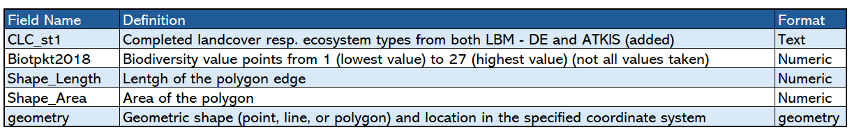
Fig. 12 Explainations of the attributes in the dataset#
Attribute formatting basics
When working with attributes:
Use quotes (
' ') for selecting text or numbers stored as strings (objectdtype).For numeric values (integers or floats), use them directly without quotes.
Understanding the dataset “Biotopwerte_Dresden_2018”
Germany has a wide variety of habitats, also known as biotopes. These biotopes can be of natural origin, such as those found in marine and coastal areas, inland waters, terrestrial and semi-terrestrial zones, and mountainous regions such as the Alps. However, there are also near-natural biotopes that are the result of technical or infrastructural conditions, such as small green spaces and open areas in urban environments.
Due to their specific characteristics, these biotopes can be classified into different biotope types according to uniform and distinguishable criteria.
The biodiversity indicator assesses the quality and diversity of biotope types as habitats for different species. This assessment is carried out using biotope value points ranging from 0-27, in accordance with the Federal Compensation Ordinance. These points are combined with spatial land cover data and intermittently available specialised data on ecosystem condition. This combination of data allows a comparative assessment of Germany’s ecosystem inventory in terms of both area and quality.
By applying biotope value points, a monetary valuation can also be carried out. This valuation is based on the average costs associated with the creation, development and maintenance of higher quality biotopes.
For more information, see the description on the IOER FDZ website.
Recommended citation
Syrbe, Ralf-Uwe, 2025, “Biotopwerte Dresden 2018”, https://doi.org/10.82617/ioer-fdz/HPXYJD, ioerDATA, V1
Selecting unique values#
Identifying unique values within a column is often a first step in understanding the categories or ranges present in your data.
Identifying unique values
The .unique() function returns an array of all distinct values in a specified column:
unique_groups = gdf['CLC_st1'].unique()
print("Unique land use codes:")
print(unique_groups)
Unique land use codes:
['122' '124' '511' '332' '322' '112' '111' '121' '123' '142' '132' '211'
 '133' '231' '221' '222' '141' '324' '311' '312' '313' '321' '131' '333'
 '411' '512']
Explaination: The dataset Biotopwerte_Dresden_2018 uses the land use codes from CORINE Land Cover (CLC), which are listed in the CLC_st1 column.
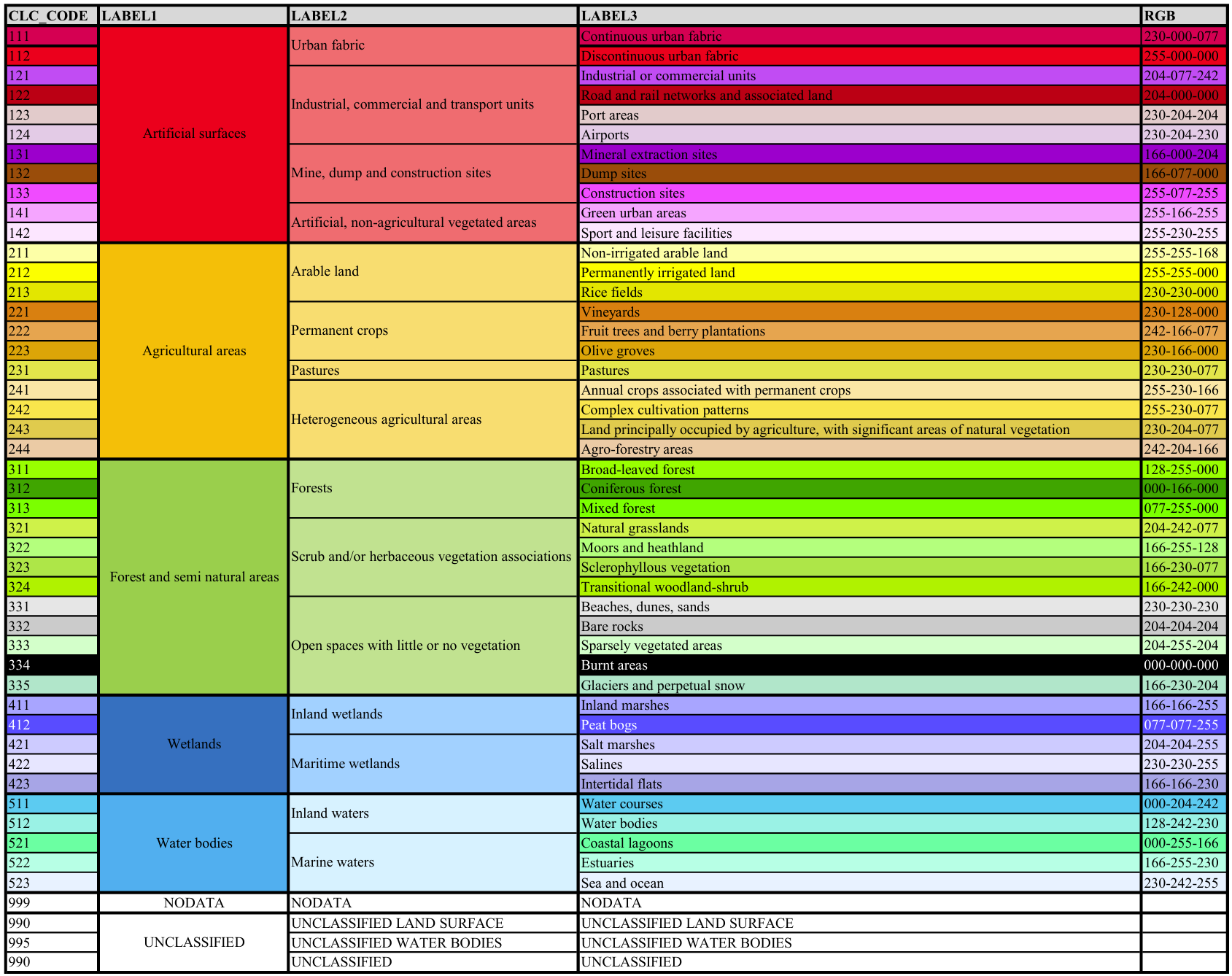
Fig. 13 Corine Land Cover (CLC) classes and their corresponding land use codes (CLC_Code). For more details, see the description of the CLC nomenclature#
Counting unique values
The .nunique() function returns the number of unique values in a column:
unique_numbers = gdf['CLC_st1'].nunique()
print(f"Number of unique land use codes: {unique_numbers}")

# Including None values in the count
unique_numbers_with_na = gdf['CLC_st1'].nunique(dropna=False)
print(f"Number of unique land use codes (including NaN): {unique_numbers_with_na}")
Number of unique land use codes: 26
Number of unique land use codes (including NaN): 26
Counting value frequencies
To see how many times each unique value appears in a column, use the .groupby() and .size() methods or the .value_counts() method.
Using .groupby() and .size():
groupcounts = gdf.groupby('CLC_st1').size()
print("\nFrequency of land use codes (using groupby):")
print(pd.DataFrame(groupcounts).T)
Frequency of land use codes (using groupby):
CLC_st1   111   112   121   122  123  124  131  132  133   141  ...   312  \
0        1115  7187  2732  5454   12  133   16   47    4  1627  ...  1546

CLC_st1   313  321  322  324  332  333  411   511  512
0        1594    8  667  525   36   10    3  2563  234

[1 rows x 26 columns]
Using value_counts:
groupcounts = gdf["CLC_st1"].value_counts()
print("\nFrequency of land use codes (using value_counts):")
pd.DataFrame(groupcounts).T
Frequency of land use codes (using value_counts):
| CLC_st1 | 112 | 122 | 231 | 121 | 511 | 142 | 311 | 141 | 313 | 312 | ... | 222 | 132 | 332 | 131 | 221 | 123 | 333 | 321 | 133 | 411 |
|---|---|---|---|---|---|---|---|---|---|---|---|---|---|---|---|---|---|---|---|---|---|
| count | 7187 | 5454 | 3293 | 2732 | 2563 | 2413 | 1787 | 1627 | 1594 | 1546 | ... | 56 | 47 | 36 | 16 | 14 | 12 | 10 | 8 | 4 | 3 |
1 rows × 26 columns
Accessing counts for specific values
You can access the frequency of a particular value directly, similar to accessing a dictionary element:
# Retrieves the count for a specific value (string format)
sv_count = groupcounts['142']
print(f"\nNumber of features with code '142': {sv_count}")
Number of features with code '142': 2413
# To group by a float-formatted column
group_2 = gdf.groupby('Biotpkt2018').size()
print("\nFrequency of biodiversity indicator values (head):")
group_2[1.000000]
Frequency of biodiversity indicator values (head):
np.int64(52)
Note: Float values must match precisely, including decimal points.
Selecting data by attribute values#
You can filter your GeoDataFrame to select only the rows that meet specific conditions based on their attribute values.
Selecting rows with a single specific value
To select rows where a column has a particular value, use boolean indexing.
Selecting by string value:
filtered_data = gdf[gdf['CLC_st1'] == '133']
print("\nFirst 5 features with CLC_st1 == '133':")
filtered_data.head(5)
Show code cell output
First 5 features with CLC_st1 == '133':
| CLC_st1 | Biotpkt2018 | Shape_Length | Shape_Area | geometry | |
|---|---|---|---|---|---|
| 11831 | 133 | 6.035751 | 17.828953 | 0.432276 | MULTIPOLYGON (((411237.019 5656164.663, 411228... |
| 24343 | 133 | 6.035751 | 287.703701 | 4278.338534 | MULTIPOLYGON (((411656.913 5656302.92, 411664.... |
| 24344 | 133 | 6.035751 | 183.544225 | 2066.507754 | MULTIPOLYGON (((411567.287 5656337.438, 411562... |
| 24347 | 133 | 6.035751 | 213.015432 | 2684.440542 | MULTIPOLYGON (((411587.489 5655959.618, 411588... |
Selecting by numeric value:
filtered_data = gdf[gdf['Biotpkt2018'] == 1.000000]
print("\nFirst 5 features with Biotpkt2018 == 1.0:")
filtered_data.head(5)
Show code cell output
First 5 features with Biotpkt2018 == 1.0:
| CLC_st1 | Biotpkt2018 | Shape_Length | Shape_Area | geometry | |
|---|---|---|---|---|---|
| 9492 | 111 | 1.0 | 411.855290 | 2480.458787 | MULTIPOLYGON (((406985.474 5655597.694, 406984... |
| 9504 | 111 | 1.0 | 89.433492 | 466.944726 | MULTIPOLYGON (((416782.224 5652196.728, 416782... |
| 9514 | 111 | 1.0 | 172.927119 | 1621.632535 | MULTIPOLYGON (((419300.05 5657313.72, 419299.9... |
| 9515 | 111 | 1.0 | 320.578260 | 3691.824728 | MULTIPOLYGON (((408302.234 5655785.262, 408296... |
| 9519 | 111 | 1.0 | 121.899927 | 920.751286 | MULTIPOLYGON (((414687.929 5655817.21, 414656.... |
Selecting rows with multiple specific values
To select rows where a column’s value is one of several specific values, use the .isin() method:
filtered_data = gdf[gdf['CLC_st1'].isin(['133', '321', '411'])]
print("\nFirst 5 features with CLC_st1 in ['133', '321', '411']:")
filtered_data.head(5)
Show code cell output
First 5 features with CLC_st1 in ['133', '321', '411']:
| CLC_st1 | Biotpkt2018 | Shape_Length | Shape_Area | geometry | |
|---|---|---|---|---|---|
| 11831 | 133 | 6.035751 | 17.828953 | 0.432276 | MULTIPOLYGON (((411237.019 5656164.663, 411228... |
| 23859 | 321 | 20.164493 | 618.702965 | 18317.038350 | MULTIPOLYGON (((415627.211 5652243.292, 415579... |
| 23860 | 321 | 20.164493 | 1099.972947 | 10894.472486 | MULTIPOLYGON (((418611.74 5653542.485, 418618.... |
| 23861 | 321 | 20.164493 | 1023.775893 | 22918.685826 | MULTIPOLYGON (((418506.559 5653953.337, 418516... |
| 23862 | 321 | 20.164493 | 1126.678849 | 17980.357862 | MULTIPOLYGON (((418145.759 5654361.049, 418151... |
Examining dataset dimensions#
The .shape attribute returns a tuple representing the number of rows and columns in your GeoDataFrame:
print(f"\nShape of filtered_data_isin: {filtered_data.shape}")
Shape of filtered_data_isin: (15, 5)
Adding new attributes (columns)#
You can add new columns to your GeoDataFrame with calculated values or constant values.
In the following example, the output of the previous step is used as the dataset, and a new column named test is added.
First, we make sure that our original dataframe is not modified by explicipty creating a copy of the dataframe.
# Ensure we are working on a copy of the data, not a view
filtered_data = filtered_data.copy()
Working on a view or copy of dataframe?
In pandas, when working with a slice of a DataFrame, you may be working on a view rather than a copy of the data. A view is simply a reference to the original DataFrame, meaning changes made to the view can affect the original data. On the other hand, a copy is a distinct, independent object, so modifications will not impact the original DataFrame. This distinction is important when assigning values to a slice because pandas will often raise a SettingWithCopyWarning to indicate that the operation might be applied to a view, leading to potential unintended side effects.
Since the dataset contains 15 rows, 15 values are assigned using the loc method. (The values could be from different formats: string, null, negative, float, integer, …)
filtered_data.loc[:, 'test']=[
    'Hello', None, -7, 4.5, 5, 6, 7, 8, 9, 10, 11, 12, 13, 14, 15]

filtered_data.head()
Show code cell output
| CLC_st1 | Biotpkt2018 | Shape_Length | Shape_Area | geometry | test | |
|---|---|---|---|---|---|---|
| 11831 | 133 | 6.035751 | 17.828953 | 0.432276 | MULTIPOLYGON (((411237.019 5656164.663, 411228... | Hello |
| 23859 | 321 | 20.164493 | 618.702965 | 18317.038350 | MULTIPOLYGON (((415627.211 5652243.292, 415579... | None |
| 23860 | 321 | 20.164493 | 1099.972947 | 10894.472486 | MULTIPOLYGON (((418611.74 5653542.485, 418618.... | -7 |
| 23861 | 321 | 20.164493 | 1023.775893 | 22918.685826 | MULTIPOLYGON (((418506.559 5653953.337, 418516... | 4.5 |
| 23862 | 321 | 20.164493 | 1126.678849 | 17980.357862 | MULTIPOLYGON (((418145.759 5654361.049, 418151... | 5 |
[ : , ‘column_name’ ]
Using : sign before comma , means selecting all the rows, and the information after comma , specifies the columns of interest.
Adding new attributes with missing values
You can initially add a column with None values and then update specific rows:
filtered_data.loc[:,'test'] = None
To update specific rows by their index:
print(filtered_data.index)
Index([11831, 23859, 23860, 23861, 23862, 23863, 23864, 24343, 24344, 24347,
       24444, 24445, 32673, 32674, 33881],
      dtype='int64')
In the following example, index 11831, 23859, and 23862 updated with their new values.
filtered_data.loc[[11831, 23859, 23862], 'test'] = \
                               [100, '200.5', 300]
filtered_data.head()
Show code cell output
| CLC_st1 | Biotpkt2018 | Shape_Length | Shape_Area | geometry | test | |
|---|---|---|---|---|---|---|
| 11831 | 133 | 6.035751 | 17.828953 | 0.432276 | MULTIPOLYGON (((411237.019 5656164.663, 411228... | 100 |
| 23859 | 321 | 20.164493 | 618.702965 | 18317.038350 | MULTIPOLYGON (((415627.211 5652243.292, 415579... | 200.5 |
| 23860 | 321 | 20.164493 | 1099.972947 | 10894.472486 | MULTIPOLYGON (((418611.74 5653542.485, 418618.... | None |
| 23861 | 321 | 20.164493 | 1023.775893 | 22918.685826 | MULTIPOLYGON (((418506.559 5653953.337, 418516... | None |
| 23862 | 321 | 20.164493 | 1126.678849 | 17980.357862 | MULTIPOLYGON (((418145.759 5654361.049, 418151... | 300 |
Adding new attributes from another dataset
Adding new attributes from another dataset is typically done through merging operations, which will be explained in the Merging Data section.
Adding new features (rows)#
You can add new rows to your GeoDataFrame using loc and providing values for all columns.
Here the index of the row is defined and for all the columns (CLC_st1, Biotpkt2018, …) the values should be assigned.
Example below creates a row with the index of sample and as the dataset includes 6 columns, 6 values defined for them.
filtered_data.loc['sample'] = ['Hello', 800, -7, 4.5, None, 9]
filtered_data.head(16)
Show code cell output
/tmp/ipykernel_2215/1904651694.py:1: FutureWarning: The behavior of DataFrame concatenation with empty or all-NA entries is deprecated. In a future version, this will no longer exclude empty or all-NA columns when determining the result dtypes. To retain the old behavior, exclude the relevant entries before the concat operation.
  filtered_data.loc['sample'] = ['Hello', 800, -7, 4.5, None, 9]
| CLC_st1 | Biotpkt2018 | Shape_Length | Shape_Area | geometry | test | |
|---|---|---|---|---|---|---|
| 11831 | 133 | 6.035751 | 17.828953 | 0.432276 | MULTIPOLYGON (((411237.019 5656164.663, 411228... | 100 |
| 23859 | 321 | 20.164493 | 618.702965 | 18317.038350 | MULTIPOLYGON (((415627.211 5652243.292, 415579... | 200.5 |
| 23860 | 321 | 20.164493 | 1099.972947 | 10894.472486 | MULTIPOLYGON (((418611.74 5653542.485, 418618.... | None |
| 23861 | 321 | 20.164493 | 1023.775893 | 22918.685826 | MULTIPOLYGON (((418506.559 5653953.337, 418516... | None |
| 23862 | 321 | 20.164493 | 1126.678849 | 17980.357862 | MULTIPOLYGON (((418145.759 5654361.049, 418151... | 300 |
| 23863 | 321 | 20.164493 | 1251.411517 | 28498.211647 | MULTIPOLYGON (((401726.203 5658676.434, 401724... | None |
| 23864 | 321 | 20.164493 | 1055.657824 | 15517.253917 | MULTIPOLYGON (((403428.145 5659215.144, 403416... | None |
| 24343 | 133 | 6.035751 | 287.703701 | 4278.338534 | MULTIPOLYGON (((411656.913 5656302.92, 411664.... | None |
| 24344 | 133 | 6.035751 | 183.544225 | 2066.507754 | MULTIPOLYGON (((411567.287 5656337.438, 411562... | None |
| 24347 | 133 | 6.035751 | 213.015432 | 2684.440542 | MULTIPOLYGON (((411587.489 5655959.618, 411588... | None |
| 24444 | 411 | 17.079406 | 389.878192 | 3208.873688 | MULTIPOLYGON (((413977.74 5649257.41, 413976.8... | None |
| 24445 | 411 | 17.079406 | 786.310517 | 17091.353830 | MULTIPOLYGON (((401901.386 5658342.569, 401914... | None |
| 32673 | 321 | 20.164493 | 755.991947 | 15304.813349 | MULTIPOLYGON (((414609.258 5667182.283, 414600... | None |
| 32674 | 321 | 20.164493 | 806.236339 | 24159.996929 | MULTIPOLYGON (((414627.453 5667492.653, 414633... | None |
| 33881 | 411 | 17.079406 | 555.046133 | 10593.540640 | MULTIPOLYGON (((411687.325 5665387.9, 411686.9... | None |
| sample | Hello | 800.000000 | -7.000000 | 4.500000 | None | 9 |
Adding new features from another dataset
Adding new features from another dataset is typically done through concatenation operations, which will be explained in the Merging Data section.
Coping data#
You can create copies of columns or rows.
Copying a column
filtered_data.loc[:,'test_2'] = filtered_data.loc[:,'test']
print("\nGeoDataFrame with a copied 'test_copied' column:")
filtered_data.head(17)
Show code cell output
GeoDataFrame with a copied 'test_copied' column:
| CLC_st1 | Biotpkt2018 | Shape_Length | Shape_Area | geometry | test | test_2 | |
|---|---|---|---|---|---|---|---|
| 11831 | 133 | 6.035751 | 17.828953 | 0.432276 | MULTIPOLYGON (((411237.019 5656164.663, 411228... | 100 | 100 |
| 23859 | 321 | 20.164493 | 618.702965 | 18317.038350 | MULTIPOLYGON (((415627.211 5652243.292, 415579... | 200.5 | 200.5 |
| 23860 | 321 | 20.164493 | 1099.972947 | 10894.472486 | MULTIPOLYGON (((418611.74 5653542.485, 418618.... | None | None |
| 23861 | 321 | 20.164493 | 1023.775893 | 22918.685826 | MULTIPOLYGON (((418506.559 5653953.337, 418516... | None | None |
| 23862 | 321 | 20.164493 | 1126.678849 | 17980.357862 | MULTIPOLYGON (((418145.759 5654361.049, 418151... | 300 | 300 |
| 23863 | 321 | 20.164493 | 1251.411517 | 28498.211647 | MULTIPOLYGON (((401726.203 5658676.434, 401724... | None | None |
| 23864 | 321 | 20.164493 | 1055.657824 | 15517.253917 | MULTIPOLYGON (((403428.145 5659215.144, 403416... | None | None |
| 24343 | 133 | 6.035751 | 287.703701 | 4278.338534 | MULTIPOLYGON (((411656.913 5656302.92, 411664.... | None | None |
| 24344 | 133 | 6.035751 | 183.544225 | 2066.507754 | MULTIPOLYGON (((411567.287 5656337.438, 411562... | None | None |
| 24347 | 133 | 6.035751 | 213.015432 | 2684.440542 | MULTIPOLYGON (((411587.489 5655959.618, 411588... | None | None |
| 24444 | 411 | 17.079406 | 389.878192 | 3208.873688 | MULTIPOLYGON (((413977.74 5649257.41, 413976.8... | None | None |
| 24445 | 411 | 17.079406 | 786.310517 | 17091.353830 | MULTIPOLYGON (((401901.386 5658342.569, 401914... | None | None |
| 32673 | 321 | 20.164493 | 755.991947 | 15304.813349 | MULTIPOLYGON (((414609.258 5667182.283, 414600... | None | None |
| 32674 | 321 | 20.164493 | 806.236339 | 24159.996929 | MULTIPOLYGON (((414627.453 5667492.653, 414633... | None | None |
| 33881 | 411 | 17.079406 | 555.046133 | 10593.540640 | MULTIPOLYGON (((411687.325 5665387.9, 411686.9... | None | None |
| sample | Hello | 800.000000 | -7.000000 | 4.500000 | None | 9 | 9 |
Copying a row
filtered_data.loc['sample_2'] = filtered_data.loc['sample']
print("\nGeoDataFrame with a copied 'sample_2' row:")
filtered_data.head(18)
Show code cell output
GeoDataFrame with a copied 'sample_2' row:
/tmp/ipykernel_2215/922061175.py:1: FutureWarning: The behavior of DataFrame concatenation with empty or all-NA entries is deprecated. In a future version, this will no longer exclude empty or all-NA columns when determining the result dtypes. To retain the old behavior, exclude the relevant entries before the concat operation.
  filtered_data.loc['sample_2'] = filtered_data.loc['sample']
| CLC_st1 | Biotpkt2018 | Shape_Length | Shape_Area | geometry | test | test_2 | |
|---|---|---|---|---|---|---|---|
| 11831 | 133 | 6.035751 | 17.828953 | 0.432276 | MULTIPOLYGON (((411237.019 5656164.663, 411228... | 100 | 100 |
| 23859 | 321 | 20.164493 | 618.702965 | 18317.038350 | MULTIPOLYGON (((415627.211 5652243.292, 415579... | 200.5 | 200.5 |
| 23860 | 321 | 20.164493 | 1099.972947 | 10894.472486 | MULTIPOLYGON (((418611.74 5653542.485, 418618.... | None | None |
| 23861 | 321 | 20.164493 | 1023.775893 | 22918.685826 | MULTIPOLYGON (((418506.559 5653953.337, 418516... | None | None |
| 23862 | 321 | 20.164493 | 1126.678849 | 17980.357862 | MULTIPOLYGON (((418145.759 5654361.049, 418151... | 300 | 300 |
| 23863 | 321 | 20.164493 | 1251.411517 | 28498.211647 | MULTIPOLYGON (((401726.203 5658676.434, 401724... | None | None |
| 23864 | 321 | 20.164493 | 1055.657824 | 15517.253917 | MULTIPOLYGON (((403428.145 5659215.144, 403416... | None | None |
| 24343 | 133 | 6.035751 | 287.703701 | 4278.338534 | MULTIPOLYGON (((411656.913 5656302.92, 411664.... | None | None |
| 24344 | 133 | 6.035751 | 183.544225 | 2066.507754 | MULTIPOLYGON (((411567.287 5656337.438, 411562... | None | None |
| 24347 | 133 | 6.035751 | 213.015432 | 2684.440542 | MULTIPOLYGON (((411587.489 5655959.618, 411588... | None | None |
| 24444 | 411 | 17.079406 | 389.878192 | 3208.873688 | MULTIPOLYGON (((413977.74 5649257.41, 413976.8... | None | None |
| 24445 | 411 | 17.079406 | 786.310517 | 17091.353830 | MULTIPOLYGON (((401901.386 5658342.569, 401914... | None | None |
| 32673 | 321 | 20.164493 | 755.991947 | 15304.813349 | MULTIPOLYGON (((414609.258 5667182.283, 414600... | None | None |
| 32674 | 321 | 20.164493 | 806.236339 | 24159.996929 | MULTIPOLYGON (((414627.453 5667492.653, 414633... | None | None |
| 33881 | 411 | 17.079406 | 555.046133 | 10593.540640 | MULTIPOLYGON (((411687.325 5665387.9, 411686.9... | None | None |
| sample | Hello | 800.000000 | -7.000000 | 4.500000 | None | 9 | 9 |
| sample_2 | Hello | 800.000000 | -7.000000 | 4.500000 | None | 9 | 9 |
Finding and handling null values#
Missing or null values are common in datasets. It’s important to identify and handle them appropriately.
Identifying columns with null values
The .isnull() method returns a boolean DataFrame indicating the presence of null values. Combining it with .any() checks if any null values exist in each column:
print("\nColumns with null values:")
filtered_data.isnull().any()
Columns with null values:
CLC_st1         False
Biotpkt2018     False
Shape_Length    False
Shape_Area      False
geometry         True
test             True
test_2           True
dtype: bool
Identifying indices of null values in a column
print("\nIndices with null values in 'test_2' column:")
filtered_data[filtered_data['test'].isnull()].index
Indices with null values in 'test_2' column:
Index([23860, 23861, 23863, 23864, 24343, 24344, 24347, 24444, 24445, 32673,
       32674, 33881],
      dtype='object')
Selecting rows with any null values
To select all rows that contain at least one null value:
print("\nRows with at least one null value:")
filtered_data[filtered_data.isnull().any(axis=1)]
Show code cell output
Rows with at least one null value:
| CLC_st1 | Biotpkt2018 | Shape_Length | Shape_Area | geometry | test | test_2 | |
|---|---|---|---|---|---|---|---|
| 23860 | 321 | 20.164493 | 1099.972947 | 10894.472486 | MULTIPOLYGON (((418611.74 5653542.485, 418618.... | None | None |
| 23861 | 321 | 20.164493 | 1023.775893 | 22918.685826 | MULTIPOLYGON (((418506.559 5653953.337, 418516... | None | None |
| 23863 | 321 | 20.164493 | 1251.411517 | 28498.211647 | MULTIPOLYGON (((401726.203 5658676.434, 401724... | None | None |
| 23864 | 321 | 20.164493 | 1055.657824 | 15517.253917 | MULTIPOLYGON (((403428.145 5659215.144, 403416... | None | None |
| 24343 | 133 | 6.035751 | 287.703701 | 4278.338534 | MULTIPOLYGON (((411656.913 5656302.92, 411664.... | None | None |
| 24344 | 133 | 6.035751 | 183.544225 | 2066.507754 | MULTIPOLYGON (((411567.287 5656337.438, 411562... | None | None |
| 24347 | 133 | 6.035751 | 213.015432 | 2684.440542 | MULTIPOLYGON (((411587.489 5655959.618, 411588... | None | None |
| 24444 | 411 | 17.079406 | 389.878192 | 3208.873688 | MULTIPOLYGON (((413977.74 5649257.41, 413976.8... | None | None |
| 24445 | 411 | 17.079406 | 786.310517 | 17091.353830 | MULTIPOLYGON (((401901.386 5658342.569, 401914... | None | None |
| 32673 | 321 | 20.164493 | 755.991947 | 15304.813349 | MULTIPOLYGON (((414609.258 5667182.283, 414600... | None | None |
| 32674 | 321 | 20.164493 | 806.236339 | 24159.996929 | MULTIPOLYGON (((414627.453 5667492.653, 414633... | None | None |
| 33881 | 411 | 17.079406 | 555.046133 | 10593.540640 | MULTIPOLYGON (((411687.325 5665387.9, 411686.9... | None | None |
| sample | Hello | 800.000000 | -7.000000 | 4.500000 | None | 9 | 9 |
| sample_2 | Hello | 800.000000 | -7.000000 | 4.500000 | None | 9 | 9 |
Removing null values
The .dropna() method removes rows or columns containing null values.
Removing rows with any null value:
print("\nGeoDataFrame after dropping rows with any null value:")
filtered_data.dropna()
Show code cell output
GeoDataFrame after dropping rows with any null value:
| CLC_st1 | Biotpkt2018 | Shape_Length | Shape_Area | geometry | test | test_2 | |
|---|---|---|---|---|---|---|---|
| 11831 | 133 | 6.035751 | 17.828953 | 0.432276 | MULTIPOLYGON (((411237.019 5656164.663, 411228... | 100 | 100 |
| 23859 | 321 | 20.164493 | 618.702965 | 18317.038350 | MULTIPOLYGON (((415627.211 5652243.292, 415579... | 200.5 | 200.5 |
| 23862 | 321 | 20.164493 | 1126.678849 | 17980.357862 | MULTIPOLYGON (((418145.759 5654361.049, 418151... | 300 | 300 |
Removing rows with null values in specific columns
print("\nGeoDataFrame after dropping rows with null in 'test' column:")
filtered_data.dropna(subset=['test'])
Show code cell output
GeoDataFrame after dropping rows with null in 'test' column:
| CLC_st1 | Biotpkt2018 | Shape_Length | Shape_Area | geometry | test | test_2 | |
|---|---|---|---|---|---|---|---|
| 11831 | 133 | 6.035751 | 17.828953 | 0.432276 | MULTIPOLYGON (((411237.019 5656164.663, 411228... | 100 | 100 |
| 23859 | 321 | 20.164493 | 618.702965 | 18317.038350 | MULTIPOLYGON (((415627.211 5652243.292, 415579... | 200.5 | 200.5 |
| 23862 | 321 | 20.164493 | 1126.678849 | 17980.357862 | MULTIPOLYGON (((418145.759 5654361.049, 418151... | 300 | 300 |
| sample | Hello | 800.000000 | -7.000000 | 4.500000 | None | 9 | 9 |
| sample_2 | Hello | 800.000000 | -7.000000 | 4.500000 | None | 9 | 9 |
Removing columns with any null value:
print("\nGeoDataFrame after dropping columns with any null value:")
filtered_data.dropna(axis=1)
Show code cell output
GeoDataFrame after dropping columns with any null value:
| CLC_st1 | Biotpkt2018 | Shape_Length | Shape_Area | |
|---|---|---|---|---|
| 11831 | 133 | 6.035751 | 17.828953 | 0.432276 |
| 23859 | 321 | 20.164493 | 618.702965 | 18317.038350 |
| 23860 | 321 | 20.164493 | 1099.972947 | 10894.472486 |
| 23861 | 321 | 20.164493 | 1023.775893 | 22918.685826 |
| 23862 | 321 | 20.164493 | 1126.678849 | 17980.357862 |
| 23863 | 321 | 20.164493 | 1251.411517 | 28498.211647 |
| 23864 | 321 | 20.164493 | 1055.657824 | 15517.253917 |
| 24343 | 133 | 6.035751 | 287.703701 | 4278.338534 |
| 24344 | 133 | 6.035751 | 183.544225 | 2066.507754 |
| 24347 | 133 | 6.035751 | 213.015432 | 2684.440542 |
| 24444 | 411 | 17.079406 | 389.878192 | 3208.873688 |
| 24445 | 411 | 17.079406 | 786.310517 | 17091.353830 |
| 32673 | 321 | 20.164493 | 755.991947 | 15304.813349 |
| 32674 | 321 | 20.164493 | 806.236339 | 24159.996929 |
| 33881 | 411 | 17.079406 | 555.046133 | 10593.540640 |
| sample | Hello | 800.000000 | -7.000000 | 4.500000 |
| sample_2 | Hello | 800.000000 | -7.000000 | 4.500000 |
Removing data#
You can remove unwanted columns or rows from your GeoDataFrame.
Removing attributes (columns)
The .drop() method removes specified columns (axis=1):
print("\nGeoDataFrame after dropping columns 'test_2' and 'CLC_st1':")
filtered_data.drop(['test_2','CLC_st1'], axis=1)
GeoDataFrame after dropping columns 'test_2' and 'CLC_st1':
| Biotpkt2018 | Shape_Length | Shape_Area | geometry | test | |
|---|---|---|---|---|---|
| 11831 | 6.035751 | 17.828953 | 0.432276 | MULTIPOLYGON (((411237.019 5656164.663, 411228... | 100 |
| 23859 | 20.164493 | 618.702965 | 18317.038350 | MULTIPOLYGON (((415627.211 5652243.292, 415579... | 200.5 |
| 23860 | 20.164493 | 1099.972947 | 10894.472486 | MULTIPOLYGON (((418611.74 5653542.485, 418618.... | None |
| 23861 | 20.164493 | 1023.775893 | 22918.685826 | MULTIPOLYGON (((418506.559 5653953.337, 418516... | None |
| 23862 | 20.164493 | 1126.678849 | 17980.357862 | MULTIPOLYGON (((418145.759 5654361.049, 418151... | 300 |
| 23863 | 20.164493 | 1251.411517 | 28498.211647 | MULTIPOLYGON (((401726.203 5658676.434, 401724... | None |
| 23864 | 20.164493 | 1055.657824 | 15517.253917 | MULTIPOLYGON (((403428.145 5659215.144, 403416... | None |
| 24343 | 6.035751 | 287.703701 | 4278.338534 | MULTIPOLYGON (((411656.913 5656302.92, 411664.... | None |
| 24344 | 6.035751 | 183.544225 | 2066.507754 | MULTIPOLYGON (((411567.287 5656337.438, 411562... | None |
| 24347 | 6.035751 | 213.015432 | 2684.440542 | MULTIPOLYGON (((411587.489 5655959.618, 411588... | None |
| 24444 | 17.079406 | 389.878192 | 3208.873688 | MULTIPOLYGON (((413977.74 5649257.41, 413976.8... | None |
| 24445 | 17.079406 | 786.310517 | 17091.353830 | MULTIPOLYGON (((401901.386 5658342.569, 401914... | None |
| 32673 | 20.164493 | 755.991947 | 15304.813349 | MULTIPOLYGON (((414609.258 5667182.283, 414600... | None |
| 32674 | 20.164493 | 806.236339 | 24159.996929 | MULTIPOLYGON (((414627.453 5667492.653, 414633... | None |
| 33881 | 17.079406 | 555.046133 | 10593.540640 | MULTIPOLYGON (((411687.325 5665387.9, 411686.9... | None |
| sample | 800.000000 | -7.000000 | 4.500000 | None | 9 |
| sample_2 | 800.000000 | -7.000000 | 4.500000 | None | 9 |
Removing features (rows)#
The .drop() method also removes specified rows by their index:
print("\nGeoDataFrame after dropping the first row and 'sample' row:")
filtered_data.drop([11831,'sample'])
Show code cell output
GeoDataFrame after dropping the first row and 'sample' row:
| CLC_st1 | Biotpkt2018 | Shape_Length | Shape_Area | geometry | test | test_2 | |
|---|---|---|---|---|---|---|---|
| 23859 | 321 | 20.164493 | 618.702965 | 18317.038350 | MULTIPOLYGON (((415627.211 5652243.292, 415579... | 200.5 | 200.5 |
| 23860 | 321 | 20.164493 | 1099.972947 | 10894.472486 | MULTIPOLYGON (((418611.74 5653542.485, 418618.... | None | None |
| 23861 | 321 | 20.164493 | 1023.775893 | 22918.685826 | MULTIPOLYGON (((418506.559 5653953.337, 418516... | None | None |
| 23862 | 321 | 20.164493 | 1126.678849 | 17980.357862 | MULTIPOLYGON (((418145.759 5654361.049, 418151... | 300 | 300 |
| 23863 | 321 | 20.164493 | 1251.411517 | 28498.211647 | MULTIPOLYGON (((401726.203 5658676.434, 401724... | None | None |
| 23864 | 321 | 20.164493 | 1055.657824 | 15517.253917 | MULTIPOLYGON (((403428.145 5659215.144, 403416... | None | None |
| 24343 | 133 | 6.035751 | 287.703701 | 4278.338534 | MULTIPOLYGON (((411656.913 5656302.92, 411664.... | None | None |
| 24344 | 133 | 6.035751 | 183.544225 | 2066.507754 | MULTIPOLYGON (((411567.287 5656337.438, 411562... | None | None |
| 24347 | 133 | 6.035751 | 213.015432 | 2684.440542 | MULTIPOLYGON (((411587.489 5655959.618, 411588... | None | None |
| 24444 | 411 | 17.079406 | 389.878192 | 3208.873688 | MULTIPOLYGON (((413977.74 5649257.41, 413976.8... | None | None |
| 24445 | 411 | 17.079406 | 786.310517 | 17091.353830 | MULTIPOLYGON (((401901.386 5658342.569, 401914... | None | None |
| 32673 | 321 | 20.164493 | 755.991947 | 15304.813349 | MULTIPOLYGON (((414609.258 5667182.283, 414600... | None | None |
| 32674 | 321 | 20.164493 | 806.236339 | 24159.996929 | MULTIPOLYGON (((414627.453 5667492.653, 414633... | None | None |
| 33881 | 411 | 17.079406 | 555.046133 | 10593.540640 | MULTIPOLYGON (((411687.325 5665387.9, 411686.9... | None | None |
| sample_2 | Hello | 800.000000 | -7.000000 | 4.500000 | None | 9 | 9 |
Filtering data based on ranges#
For numeric attributes, you can filter data based on specific ranges.
To find the minimum and maximum values of the features, the following code is used:
min: minimum value in the specified attributemax: maximum value in the specified attribute
min_value = gdf['Shape_Area'].min()
max_value = gdf['Shape_Area'].max()
print(f"minimum: {min_value:0.8f}") # 0.8f round the number to 8 decimals
print(f"maximum: {max_value:0.2f}") # 0.2f round the number to 2 decimals
minimum: 0.00000562
maximum: 3249895.12
For example, it can be decided to work only with the features having areas less than 1000.
# Filter features with Shape_Area less than 1000
filter_db = gdf[gdf['Shape_Area'] < 1000]
print("\nFirst 5 features with Shape_Area less than 1000:")
filter_db.head()
Show code cell output
First 5 features with Shape_Area less than 1000:
| CLC_st1 | Biotpkt2018 | Shape_Length | Shape_Area | geometry | |
|---|---|---|---|---|---|
| 1 | 122 | 5.271487 | 31.935928 | 50.075513 | MULTIPOLYGON (((417850.525 5650376.33, 417846.... |
| 3 | 122 | 5.271487 | 24.509066 | 36.443441 | MULTIPOLYGON (((423453.146 5650332.06, 423453.... |
| 4 | 122 | 5.271487 | 29.937138 | 40.494155 | MULTIPOLYGON (((417331.434 5650889.039, 417330... |
| 6 | 122 | 5.271487 | 390.293053 | 764.349833 | MULTIPOLYGON (((407613.154 5651943.2, 407618.7... |
| 7 | 122 | 5.271487 | 34.931619 | 45.486260 | MULTIPOLYGON (((416066.508 5651463.834, 416066... |
The visualization of this filtered data will be covered in the Creating Maps section.