Clipping Data

Clipping Data#

Clipping is a process used to extract specific parts of data based on a predefined dataset that represents the area of interest. The geopandas and matplotlib packages are used for this process.

import geopandas as gp
import matplotlib.pyplot as plt
from pathlib import Path

INPUT = Path.cwd().parents[0] / "00_data"
OUTPUT = Path.cwd().parents[0] / "out"
OUTPUT.mkdir(exist_ok=True)

gdb_path = INPUT / "Biotopwerte_Dresden_2018.gdb"

Clipping Based on Zone (Dataset)#

The areas of interest in this chapter are districts in Dresden.

Dresden Portal!

The districts are extracted from the Portal of Dresden.

For retrieving the data, from the Geojson section of the portal, based on the interested format, the URL is chosen.

geojson_url = "https://kommisdd.dresden.de/net4/public/ogcapi/collections/L137/items"

Then the requests library is imported and a request is sent to the portal to extract the data.

import requests

response = requests.get(geojson_url)

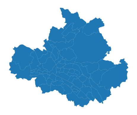
Then if the request is successful (code 200), it will load and plot the data.

if response.status_code == 200:
    gdf = gp.read_file(geojson_url)
    print(gdf.head())
    ax=gdf.plot()
    ax.set_axis_off()
else:
    print("Error:", response.text)

Selecting the area of interest!

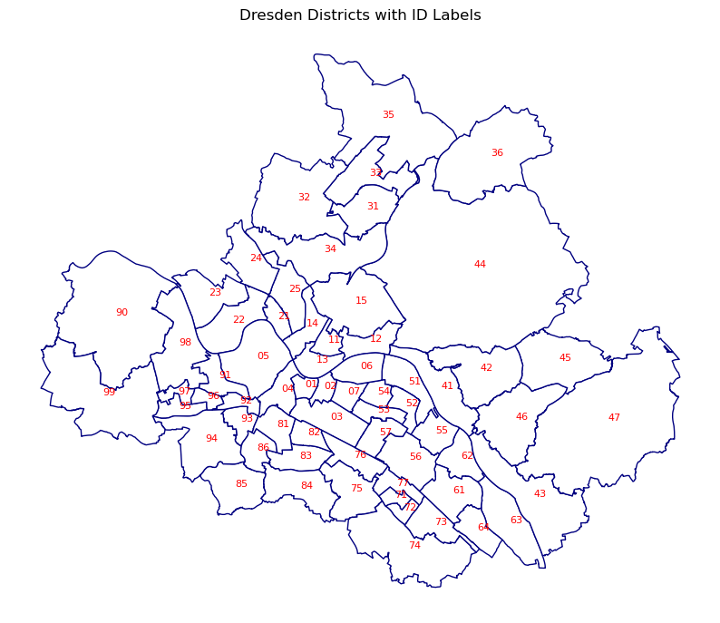
To select the area of interest, the methods mentioned in the Selecting and Filtering Chapter could be used, but also it is possible to add the labels to maps and select based on labels.

To add the labels, first, the position of the labels should be defined.

The centroid of the polygons would be the position of the labels and is generated using the geometry.centroid method and stored in a new column.

gdf["centroid"] = gdf.geometry.centroid 

/tmp/ipykernel_2419/1565410799.py:1: UserWarning: Geometry is in a geographic CRS. Results from 'centroid' are likely incorrect. Use 'GeoSeries.to_crs()' to re-project geometries to a projected CRS before this operation.

  gdf["centroid"] = gdf.geometry.centroid

For adding the labels the text function is used.

The coordinates of the centroid are the position of the labels and the label text is defined with str. In the following example, the IDs of the districts are used.

Labels in the map!

To customize the labels more, check here.

fig, ax = plt.subplots(figsize=(10, 10))
gdf.plot(ax=ax, color='white', edgecolor='navy')
ax.set_axis_off()

for idx, row in gdf.iterrows():
    plt.text(row.centroid.x, row.centroid.y, str(row['id']),
             fontsize=8, 
             color='red')

plt.title("Dresden Districts with ID Labels")
plt.show()

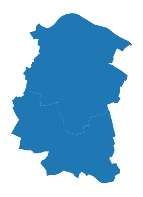
../_images/5b5004adf0c77ef19cc547f47700b10b3a745b3a1f6305cdea3a0a5779e47b01.png

Now using the labels the interested area is selected.

clipping_dataset= gdf[gdf['id'].isin(['90','99'])]
ax=clipping_dataset.plot()
ax.set_axis_off()

../_images/f705df3d240a140f5cf9af9ce0fdb06dda19158f8f90b5d5a018663c922dc4ce.png

The path to the original dataset and the clipping dataset, based on which the original dataset should be clipped, will be defined.

original_dataset = gp.read_file(gdb_path, layer="Biotopwerte_Dresden_2018")

/opt/conda/envs/worker_env/lib/python3.13/site-packages/pyogrio/raw.py:198: RuntimeWarning: organizePolygons() received a polygon with more than 100 parts. The processing may be really slow.  You can skip the processing by setting METHOD=SKIP, or only make it analyze counter-clock wise parts by setting METHOD=ONLY_CCW if you can assume that the outline of holes is counter-clock wise defined
  return ogr_read(

The coordinate system of the datasets is checked. If the coordinate systems do not match, the clipping process will not proceed.

original_dataset.crs

<Projected CRS: EPSG:25833>
Name: ETRS89 / UTM zone 33N
Axis Info [cartesian]:
- E[east]: Easting (metre)
- N[north]: Northing (metre)
Area of Use:
- name: Europe between 12°E and 18°E: Austria; Croatia; Denmark - offshore and offshore; Germany - onshore and offshore; Italy - onshore and offshore; Norway including Svalbard - onshore and offshore.
- bounds: (12.0, 34.79, 18.01, 84.01)
Coordinate Operation:
- name: UTM zone 33N
- method: Transverse Mercator
Datum: European Terrestrial Reference System 1989 ensemble
- Ellipsoid: GRS 1980
- Prime Meridian: Greenwich

clipping_dataset.crs

<Geographic 2D CRS: EPSG:4326>
Name: WGS 84
Axis Info [ellipsoidal]:
- Lat[north]: Geodetic latitude (degree)
- Lon[east]: Geodetic longitude (degree)
Area of Use:
- name: World.
- bounds: (-180.0, -90.0, 180.0, 90.0)
Datum: World Geodetic System 1984 ensemble
- Ellipsoid: WGS 84
- Prime Meridian: Greenwich

If the coordinate systems are not the same, they are transformed to match.

clipping_dataset = clipping_dataset.to_crs('EPSG:25833')

The dataset is then clipped by defining the original dataset and the clipping dataset using the clip function in the geopandas package.

clipped_dataset = gp.clip(original_dataset, clipping_dataset)

And the result of the clip operation will be printed out.

clipped_dataset.head(3)

	CLC_st1	Biotpkt2018	Shape_Length	Shape_Area	geometry
261	122	5.271487	1765.048621	6984.236836	POLYGON ((404092.96 5654379.53, 404098.204 565...
5928	322	18.055116	204.848619	582.329680	POLYGON ((404867.05 5654106.356, 404862.483 56...
13027	142	7.000000	481.434416	11886.564349	POLYGON ((405339.13 5654136.481, 405172.058 56...

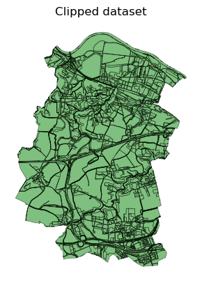
ax = clipped_dataset.plot(color="green", linewidth=0.5, alpha=0.5, edgecolor="black")
ax.set_title("Clipped dataset")
ax.set_axis_off()

../_images/f3d9a34602661ff58c8db5baf432b0941d0c8060aa8938b2a789112d1b0a13d6.png

The result can be saved in various formats. All you need to do is define the output path and export based on the format you are interested in.

Shapefile Format

output_shp = OUTPUT / "clipped.shp"
clipped_dataset.to_file(output_shp)

/tmp/ipykernel_2419/1343647297.py:2: UserWarning: Column names longer than 10 characters will be truncated when saved to ESRI Shapefile.
  clipped_dataset.to_file(output_shp)
/opt/conda/envs/worker_env/lib/python3.13/site-packages/pyogrio/raw.py:723: RuntimeWarning: Normalized/laundered field name: 'Biotpkt2018' to 'Biotpkt201'
  ogr_write(
/opt/conda/envs/worker_env/lib/python3.13/site-packages/pyogrio/raw.py:723: RuntimeWarning: Normalized/laundered field name: 'Shape_Length' to 'Shape_Leng'
  ogr_write(

GeoPackage Format

output_gdb = OUTPUT / "clipped.gpkg"
clipped_dataset.to_file(
    output_gdb,
    layer="clipped_dataset",
    driver="GPKG")

CSV Format or WKT Format

Geometry as WKT

Our data is already in WKT format. If the dataset doesn’t have a geometry column in Well Known Text format, it should be converted first, as mentioned in the next steps. You will see in the final CSV file saved below that the two columns “geometry” and “geometry_wkt” match.

Have a look at the geometry column, which commonly exists for GeoDataFrames

clipped_dataset.geometry

First, ensure that the geometry column contains valid geometries. We need to check if all values in clipped_dataset["geometry"] are actual shapely.geometry objects.

Check if there are any missing geometries (.isna()).

print(clipped_dataset["geometry"].isna().sum())  # Count missing values

Check the types of geometries.

print(clipped_dataset.geom_type.value_counts())

Polygon         2833
MultiPolygon      90
Name: count, dtype: int64

Explicitly store WKT geometries in a new column. This uses the apply function with a lambda expression to convert each geometry in the column to a string format.

from shapely.geometry import Polygon, MultiPolygon

clipped_dataset["geometry_wkt"] = clipped_dataset["geometry"].apply(
    lambda geom: geom.wkt if isinstance(geom, (Polygon, MultiPolygon)) else None
)

The output path is defined, and the data is saved as a CSV file. If the index column, which represents unique values for rows, is not needed, the index parameter can be set to False.

Parameters for CSV file

To learn how to customize your CSV data, visit the pandas DataFrame to CSV page.

csv_path = OUTPUT / "clipped_dataset.csv"
clipped_dataset.to_csv(csv_path, index=True)

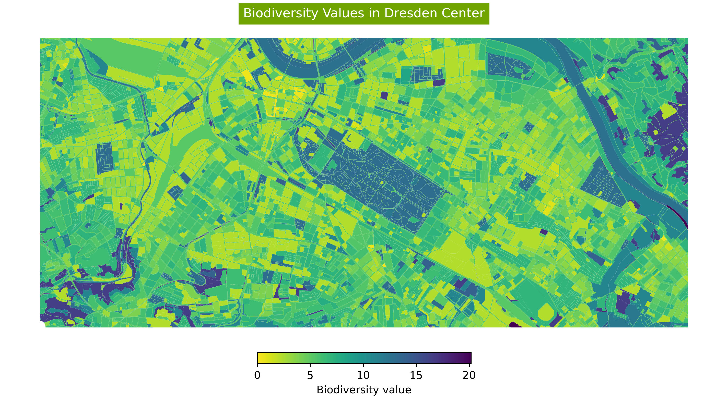
Clipping Based on Bounding Box#

To show a specific area of the dataset, the data can be clipped to a defined bounding box and then visualized.

For this reason, the required part of the dataset is selected and the bounding box is extracted for this rows.

Bounding Box

The bounding box extraction explained more in Creating Maps Chapter.

required_part= original_dataset[80:120].total_bounds

Then the dataset clipped for plotting:

gdf_clipped = gp.clip(original_dataset, required_part)

fig, ax = plt.subplots(
    nrows=1, ncols=1, figsize=(12, 18), dpi=300)

ax = gdf_clipped.plot(
    ax=ax,
    column='Biotpkt2018', 
    cmap='viridis_r',
    legend=True,
    legend_kwds={
        "label": "Biodiversity value", "orientation": "horizontal",
        "shrink": 0.3, "pad": 0.01})

ax.set_title('Biodiversity Values in Dresden Center',
             backgroundcolor='#70A401',
             color='white')
ax.set_axis_off()

../_images/d9b5a54be62b258b482f2917b1947d0d78dcdc8eefed894c8a495ff7b1378fcc.png

Clipping Data

Contents

Clipping Data#

Clipping Based on Zone (Dataset)#

Clipping Based on Bounding Box#